


Correlation Analysis
In correlation analysis, we estimate a sample correlation coefficient, more specifically the Pearson Product Moment correlation coefficient. The sample correlation coefficient, denoted r,
ranges between -1 and +1 and quantifies the direction and strength of the linear association between the two variables. The correlation between two variables can be positive (i.e., higher levels of one variable are associated with higher levels of the other) or negative (i.e., higher levels of one variable are associated with lower levels of the other).
The sign of the correlation coefficient indicates the direction of the association. The magnitude of the correlation coefficient indicates the strength of the association.
For example, a correlation of r = 0.9 suggests a strong, positive association between two variables, whereas a correlation of r = -0.2 suggest a weak, negative association. A correlation close to zero suggests no linear association between two continuous variables.
It is important to note that there may be a non-linear association between two continuous variables, but computation of a correlation coefficient does not detect this. Therefore, it is always important to evaluate the data carefully before computing a correlation coefficient. Graphical displays are particularly useful to explore associations between variables.
The figure below shows four hypothetical scenarios in which one continuous variable is plotted along the X-axis and the other along the Y-axis.
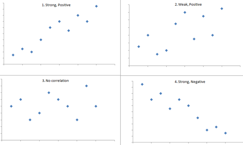
- Scenario 1 depicts a strong positive association (r=0.9), similar to what we might see for the correlation between infant birth weight and birth length.
- Scenario 2 depicts a weaker association (r=0,2) that we might expect to see between age and body mass index (which tends to increase with age).
- Scenario 3 might depict the lack of association (r approximately = 0) between the extent of media exposure in adolescence and age at which adolescents initiate sexual activity.
- Scenario 4 might depict the strong negative association (r= -0.9) generally observed between the number of hours of aerobic exercise per week and percent body fat.

Example - Correlation of Gestational Age and Birth Weight
A small study is conducted involving 17 infants to investigate the association between gestational age at birth, measured in weeks, and birth weight, measured in grams.
|
Infant ID # |
Gestational Age (weeks) |
Birth Weight (grams) |
|---|---|---|
|
1 |
34.7 |
1895 |
|
2 |
36.0 |
2030 |
|
3 |
29.3 |
1440 |
|
4 |
40.1 |
2835 |
|
5 |
35.7 |
3090 |
|
6 |
42.4 |
3827 |
|
7 |
40.3 |
3260 |
|
8 |
37.3 |
2690 |
|
9 |
40.9 |
3285 |
|
10 |
38.3 |
2920 |
|
11 |
38.5 |
3430 |
|
12 |
41.4 |
3657 |
|
13 |
39.7 |
3685 |
|
14 |
39.7 |
3345 |
|
15 |
41.1 |
3260 |
|
16 |
38.0 |
2680 |
|
17 |
38.7 |
2005 |
We wish to estimate the association between gestational age and infant birth weight. In this example, birth weight is the dependent variable and gestational age is the independent variable. Thus y=birth weight and x=gestational age. The data are displayed in a scatter diagram in the figure below.
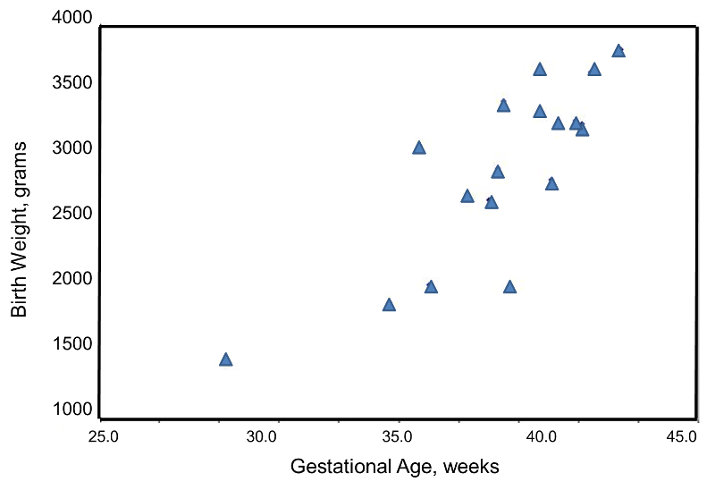
Each point represents an (x,y) pair (in this case the gestational age, measured in weeks, and the birth weight, measured in grams). Note that the independent variable, gestational age) is on the horizontal axis (or X-axis), and the dependent variable (birth weight) is on the vertical axis (or Y-axis). The scatter plot shows a positive or direct association between gestational age and birth weight. Infants with shorter gestational ages are more likely to be born with lower weights and infants with longer gestational ages are more likely to be born with higher weights.