


Cohort Studies and Case-Control Studies
The cohort study design identifies a people exposed to a particular factor and a comparison group that was not exposed to that factor and measures and compares the incidence of disease in the two groups. A higher incidence of disease in the exposed group suggests an association between that factor and the disease outcome. This study design is generally a good choice when dealing with an outbreak in a relatively small, well-defined source population, particularly if the disease being studied was fairly frequent.
The case-control design uses a different sampling strategy in which the investigators identify a group of individuals who had developed the disease (the cases) and a comparison of individuals who did not have the disease of interest. The cases and controls are then compared with respect to the frequency of one or more past exposures. If the cases have a substantially higher odds of exposure to a particular factor compared to the control subjects, it suggests an association. This strategy is a better choice when the source population is large and ill-defined, and it is particularly useful when the disease outcome was uncommon. Examples of two real outbreaks will be used to illustrate these differences in sampling strategy.
Example of a Cohort Study
A community in Massachusetts experienced an outbreak of Salmonellosis. Health officials noted that an unusually large number of cases had been reported during a span of several days. The table below summarizes some of the salient facts about Salmonella infections. Descriptive epidemiology was conducted, and hypothesis-generating interviews indicated that all of the disease people had attended a parent-teacher luncheon at a local school. In fact, it was a potluck luncheon, and the attendees each brought a dish that they had either prepared at home or purchased. The descriptive epidemiology convincingly indicated that the outbreak originated at the luncheon, but which specific dish was responsible? The investigators needed to establish which dish was responsible in order to clearly establish the source and to ensure that appropriate control measures were undertaken.
|
Salmonella Incubation period: 1-3 days
Symptoms: Diarrhea, fever, abdominal cramps, vomiting. S. Typhi and S. Paratyphi produce typhoid with insidious onset characterized by fever, headache, constipation, malaise, chills, myalgia; diarrhea is uncommon and vomiting is usually not severe.
Duration: 4-7 days
Sources: Contaminated eggs, poultry, unpasteurized milk or juice, cheese, contaminated raw fruits and vegetables (alfalfa sprouts, melons). S. Typhi epidemics are often related to fecal contamination of water supplies or street vended food. Other sources include pet rodents (hamsters, mice, and rats, or their bedding) and reptiles and amphibians (e.g., turtles, frogs, snakes, lizards, iguanas, etc.)
Laboratory Confirmation: Stool cultures
|
The source population was obviously the attendees of the luncheon, and 58% of the attendees had developed symptoms consistent with the case definition. Of these, 45 attendees agreed to complete a questionnaire regarding the foods that they had eaten at the luncheon. Since they had a relatively small, discrete cohort and a fairly high incidence of disease, a cohort design was a logical choice. For each dish served at the luncheon the investigators compared the incidence of Salmonellosis between those who ate a particular dish (the exposed group) and those who had not eaten that dish (the non-exposed comparison group). For each dish they constructed a contingency table to summarize the result from the survey. For example, the table below summarizes the findings from the survey regarding the incidence of disease in those who ate the cheese appetizer compared to those who did not eat it.
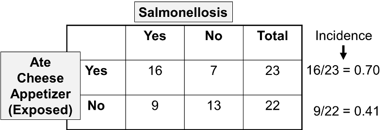
These results indicate that 23 attendees recalled eating the cheese appetizer, and 16 of them subsequently developed Salmonellosis, i.e., an incidence of 70%. There were 22 attendees who did not recall eating the cheese appetizer, and 9 or these developed symptoms of Salmonellosis, for an incidence of 41%.
When comparing the incidence of disease in an exposed group and an unexposed group, the magnitude of association is often summarized by computing a risk ratio, as follows.
Risk Ratio = (Incidence in the exposed group) / (Incidence in the unexposed group)
Therefore, for the Salmonella outbreak:
Risk Ratio = (16/23)/(9/22) = 0.70/0.41 = 1.70
This provides a means of estimating the magnitude of association between eating the cheese appetizer and risk of getting Salmonellosis. In order to complete the analysis, the investigators performed these computations for each of the dishes served at the luncheon. The table below summarizes all of the findings.
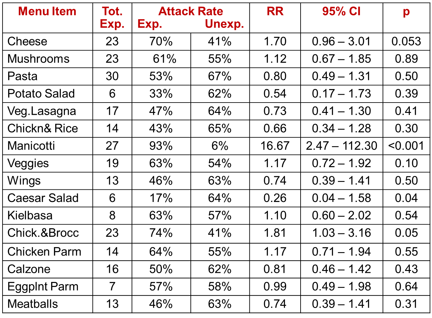
If there were no association between a particular exposure and risk of disease, then we would expect a risk ratio = 1.0. However, the overall sample was very small, and some of the dishes had very few takers, such as the potato salad. It is not surprising then that the risk ratios (column "RR") vary above and below a value of 1 as a result of random error (i.e., sampling error). One can assess the extent of random error by computing a 95% confidence interval for each estimated risk ratio (see the next to last column), and we can also compute a "p" value, as shown in the last column. A common interpretation of a 95% confidence interval for a risk ratio is that it is the range within which the true RR is likely to fall with 95% confidence. Conversely, the true value is unlikely to lie outside this range. The confidence interval also provides a measure of the precision of the estimated risk ratio. The p value is the probability of observing a difference between the exposed and unexposed groups this larger or larger if the groups truly didn't differ. The last three columns, then, help us put all of this into perspective. Most of the risk ratios (RR) are somewhat above or below a value of 1.0, which would indicate no difference. However, the risk ratio for exposure to manicotti was 16.67, suggesting that those who ate the manicotti had almost 17 times the risk of developing Salmonellosis. The 95% confidence interval for manicotti was very wide, but the lower limit of the interval was 2.47, suggesting that it is unlikely that the risk was less than 2.5-fold. Finally, the p value was less than 0.001, which indicates a very low probability that the difference was the result of random error. It would, therefore, be reasonable to conclude that the manicotti was the source of the Salmonella outbreak.
For more information about cohort studies, risk ratios, confidence intervals, and p values, please consult the following modules:
- Link to module on Measures of Association
- Link to modules on Random Error
- Link to module on Cohort Studies