Outbreak Investigations
An outbreak is essentially the same thing as an epidemic, i.e., an increased frequency of a disease above the usual rate (endemic rate) in a given population or geographic area. Pandemic refers to simultaneous epidemics occurring in multiple locations across the globe. Traditionally, these terms referred to infectious diseases, but they can also be used to describe non-infectious diseases and chronic conditions, such as lung cancer and obesity. In addition, the principles of investigation are similar for all of these. This module provides a practical introduction to the steps involved in outbreak investigations, and it provides some useful tools.
After successfully completing this section, the student will be able to:
- Labeling columns and rows & entering text and numeric data.
- Sorting data.
- Using Excel functions to tabulate data using the COUNT and SUM functions to tabulate data.
A Salmonella Outbreak after a School Luncheon – A Cohort Study
The Hepatitis A Outbreak in Marshfield, MA – A Case-Control Study
Outbreaks generally come to the attention of state or local health departments in one of two ways:
For more information, see the online learning module on Surveillance.
The primary reason for conducting outbreak investigations is to identify the source in order to establish control and to institute measures that will prevent future episodes of disease. They are also sometimes undertaken to train new personnel or to learn more about the disease and its mechanisms for transmission. Whether an outbreak investigation will be conducted may also be influenced by the severity of the disease, the potential for spread, the availability of resources, and sometimes by political considerations or the level of concern among the general public.
Most outbreak investigations involve the following steps:
Some of the steps may be conducted simultaneously, and the order may vary depending on the circumstances. For example, if new cases are continuing to occur and there are steps that can be taken to control the outbreak and prevent more cases, then certainly control and prevention measures would take top priority.
Before embarking on an outbreak investigation, consider necessary preparations:
We noted that an outbreak is an increase in the frequency of a disease above what is expected in a given population. However, an apparent outbreak can result from either incorrect diagnoses, multiple diseases with similar symptoms, or even changes in record keeping or surveillance practices. It is important to establish that the outbreak is real by examining how the cases were diagnosed and by determining what the baseline rate of disease was previously. For reportable diseases, baseline rates of disease (i.e., the usual or expected rate) can be determined from surveillance data, and you can compare rates during the previous month or weeks with the current rates of disease. For non-reportable diseases or conditions you may be able to find baseline data from state or national vital statistics, from disease registries, or from hospital discharge records, such as the Massachusetts Health Data Consortium. If you have detailed data on the number of cases of disease over time, an epidemic curve is an informative way to display this data graphically, and an epidemic curve can also provide clues about the source of infectious disease outbreaks, as we will see later.

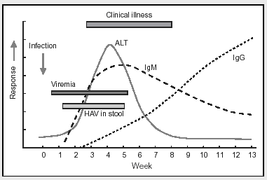
Anti-HAV antibodies of the IgM class rise very promptly after infection with the virus, even before symptoms occur. Over time IgM anti-HAV antibodies decline and are progressively replaced by the anti-HAV IgG antibodies that confer long-lasting immunity to HAV. Therefore, high titers of IgM anti-HAV indicate recent infection, while high titers of IgG anti-HAV indicate that the individual was infected in the past and is now immune. For more detailed instruction on the use of serological tests for hepatitis, please see CDC's Online Serology Training.
For more information on laboratory testing see the following from the Focus on Epidemiology series:
By a case definition we mean the standard criteria for categorizing an individual as a case. Establishing a case definition (the criteria that need to be met in order to be considered "a case") can be tricky, particularly in the initial phases of the investigation. You want your definition to specific enough to identify true cases of disease, but you also want it to be broad enough and sensitive enough that it will identify most, if not all of the cases. As a result, the case definition may change during the investigation. In the earliest stages, it might be broader and less specific in order to make sure you identify all of the potential cases ("possible" cases), but later on, it might include more specific clinical or laboratory criteria that enable you to categorize individuals as "probable" or "confirmed" cases.
Case definitions may include four types of information:
The CDC also makes well established case definitions available:
Clinical description
An illness caused by the protozoan Giardia lamblia and characterized by diarrhea, abdominal cramps, bloating, weight loss, or malabsorption. Infected persons may be asymptomatic.
Laboratory criteria for diagnosis
Case classification
Clinical case definition
An illness with a) discrete onset of symptoms and b) jaundice or elevated serum aminotransferase levels
Laboratory criteria for diagnosis
Case classification
Comment: A serologic test for IgG antibody to the recently described hepatitis C virus is available, and many cases of non-A, non-B hepatitis may be demonstrated to be due to infection with the hepatitis C virus. With this assay, however, a prolonged interval between onset of disease and detection of antibody may occur. Until a more specific test for acute hepatitis C becomes available, these cases should be reported as non-A, non-B hepatitis. Chronic carriage or chronic hepatitis should not be reported.
These should be simple, objective, and discriminating (i.e. able to distinguish between people with disease and those without disease. For example,
Also, case definitions should not include risk factors that you may want to evaluate, since all of the cases would have the risk factor, and this would be misleading. A case definition is not the same as a clinical diagnosis. Case definitions are an aid to conducting an epidemiologic investigation, whereas a clinical diagnosis is used to make treatment decisions for individual patients.
Sometimes investigators will use a loose definition early on to help them identity the extent of the outbreak. However, once the investigation progresses to the stage of conducting analytic studies to test hypotheses, a more specific definition should be used in order to reduce misclassification which would bias the results.
Once a case definition has been established, there should be a concerted effort to identify as many cases as possible in order to accurately establish the magnitude and scope of the outbreak. The cases that are reported to the state and local health departments may represent only a small fraction of the total cases for the outbreak. Therefore, in addition to cases identified via passive surveillance (i.e., cases that self-report or are reported to the state and local health department by physicians' offices, clinics, hospitals, and laboratories) it is often fruitful to conduct active surveillance by calling hospitals, laboratories, clinics, and physicians offices in order to identify potential cases that otherwise would have gone unreported. As cases are identified, it can also be useful to ask them if they know of others who are similarly affected, e.g., family members and acquaintances. Occasionally, investigators will try to identify cases by posting notices in the media. These serve the dual purpose of alerting the public about potential hazards and identifying possible cases that have already become ill. For more information on case finding see Case Finding and Line Listing: A Guide for Investigators.
Descriptive epidemiology focuses on "person, place, and time", i.e., the personal characteristics of the cases, changes in disease frequency over time, and differences in disease frequency based on location. Characteristics of person, place, and time are the essential elements of for both descriptive epidemiology (to identify possible sources) and for analytic epidemiology (to definitively identify the source).
As cases are identified it is important to record information in a systematic way and to organize it in a way that will make analysis much easier. Traditionally, the data collected during outbreak investigations was recorded on paper in a "line listing", with each case on a separate row and with the items of information in columns. However, it is much easier to record information in an electronic spreadsheet such as Excel, and this will make it much easier to work with the data, since we will show you how to use Excel to sort the data, create an epidemic curve, and compute tallies that will make the descriptive analysis and the analytical analysis a snap. A spreadsheet makes it easy to create a matrix or table which lists information about each case in a row, with columns for each of the variables of interest (e.g., name, gender, age, address, occupation, laboratory findings, relevant exposures, and columns for each of the symptoms that have been included in the case definition, etc.)
Since the investigation will hinge on an analysis of factors related to person, place, and time, the following information should be collected from cases:
- Sources of food (especially ready to eat or uncooked food) and water, including restaurants, cafeterias, etc.
- Raw shellfish consumption
- Recent travel, especially to foreign countries
- Sexual contacts
When interviewing cases, this information might be entered initially onto a case report form or a questionnaire, but it will later be entered into the line listing. The table below shows the first six cases entered into a hypothetical investigation of a hepatitis A outbreak.
| Case # | Initials | Date of Report | Date of Onset | MD Dx | nausea | vomiting | anorexia | fever | dark urine | jaundice | IgM HAV | Age | Sex |
| P1 | TK | 4/6/2004 | 4/2/2004 | Hep A | 0 | 1 | 0 | 1 | 1 | 1 | + | 45 | F |
| P2 | CC | 6/20/2004 | 6/15/2004 | Hep A | 1 | 1 | 1 | 1 | 1 | 1 | + | 57 | M |
| P3 | JD | 7/7/2004 | 7/2/2004 | Hep A | 0 | 1 | 0 | 1 | 1 | 1 | + | 23 | M |
| P4 | PR | 9/5/2004 | 9/1/2004 | Hep A | 1 | 1 | 1 | 1 | 0 | 0 | + | 18 | M |
| P5 | TH | 11/29/2004 | 11/24/2004 | Hep A | 1 | 1 | 0 | 1 | 1 | 1 | + | 56 | F |
| P6 | VH | 12/19/2004 | 12/15/2004 | Hep A | 0 | 1 | 1 | 1 | 1 | 0 | + | 43 | M |
Note that each case is on a separate row, and the variables for each are entered in columns. Note also that the presence or absence of symptoms was indicated using numeric entries with 1 indicating 'yes' and 0 indicating 'no'. The use of numeric data has two great advantages. First, it is unambiguous, whereas alphanumeric entries could be "Y", "y", "YES", "Yes", "yes, "NO", "no", etc. A second major advantage to numeric entries is that they will enable us to take advantage of built in Excel functions that will make analysis of the data exceedingly easy.
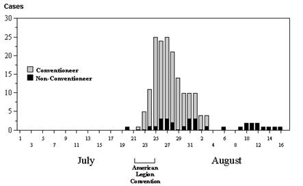 Changes in the frequency of disease over time are best illustrated with an epidemic curve, which shows the number of new cases at intervals over time. The graph to the right is an epidemic curve for the first outbreak of Legionnaires' disease in 1976 in Philadelphia.An epidemic curve provides a great deal of information. If you know what disease you are dealing with and you know its incubation period, the pattern of disease occurrence over time can narrow down the source of infection.
In essence, an epidemic curve is a bar chart with vertical columns that illustrates number of new cases of a specific disease occurring over a span of time. The key information is the time of onset for each of the cases. To construct the epidemic curve one counts up the number of new cases occurring during fixed time intervals (hours, 1 day, 2 days, 4 days, or some other interval.) The interval that is chosen will depend on the length of the time span of interest and the incubation period of the disease being investigated. A brief outbreak of salmonellosis caused by a pot luck luncheon might use 8-hour intervals because of the brevity of the outbreak and the fact that the incubation period for salmonellosis is only 1-3 days. In contrast, an epidemic of hepatitis A caused by an infected food handler at a restaurant might use 1-day or 2 day intervals because hepatitis A has an average incubation period of about 30 days. A useful rule of thumb is to use an interval that allows you to summarize the outbreak with perhaps 10-20 time intervals, as the epidemic curve for Legionnaires' disease illustrates. It is also useful to show the frequency of disease for a period of time before and after the epidemic as well in order to provide perspective.
These videos demonstarte how to construct an epidemic curve using an Excel spreadsheet. The first method is simple, but of limited use with a large sample.
The second method uses pivot tables in Excel and it is better with large samples.
An examination of the shape and duration of the epidemic curve can provide clues about the possible source as illustrated in the table below. However, epidemic curves don't always neatly conform to one of these three patterns.
Point Source Epidemic
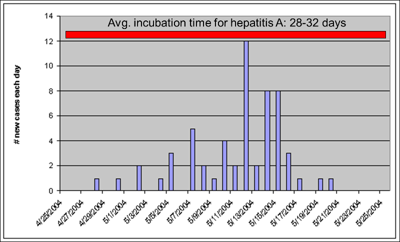
Point source epidemics have a focal source that infects a number of people during a limited period of time. A good example would be a food handler at a restaurant who has a subclinical infection with hepatitis A. The food handler would shed virus for perhaps only a few weeks. In point source epidemics the cases tend to occur during a span of time equal to the average incubation period of the disease. The illustration above shows a point source epidemic of hepatitis A in which all of the cases occur within a one month period consistent with hepatitis A's average incubation period of about 30 days.
Continuous Common Source Epidemic
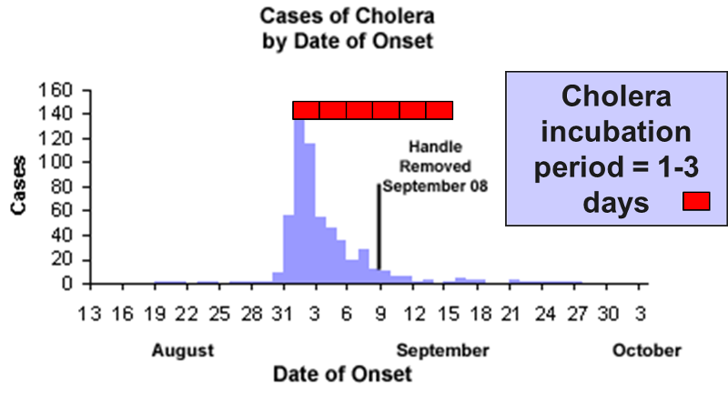
The source is prolonged over an extended period of time and may occur over more than one incubation period. The down slope of the curve may be very sharp if the common source is removed or gradual if the outbreak is allowed to exhaust itself.
The illustration depicts the outbreak of cholera that occurred in the Broad St. area of London in 1853. The source was a community well that had become contaminated with Vibrio cholerae. Cholera has an incubation period of only 1-3 days. Note however, that the epidemic lasted for more than two weeks. Cases diminished because residents fled the area, but it wasn't terminated until the pump handle was removed.
Propagated Epidemic
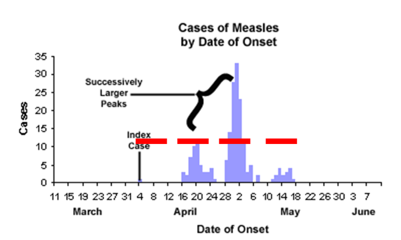
In a propagated epidemic an initial cluster of cases serves as a source of infection for subsequent cases and those subsequent cases, in turn, serve as sources for later cases. This can result in a series of successively larger peaks, reflective of the increasing number of cases caused by person-to-person contact, until the pool of susceptible people is exhausted or control measures are implemented. The figure above shows a measles outbreak in which an index case triggers a cluster of cases, and they, in turn lead to a second cluster of cases, leading finally to a third cluster.
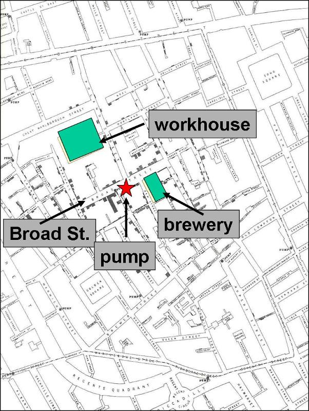
Assessing the location of cases may reveal clusters or patterns that provide clues about the source. It is sometime useful to construct a "spot map" of the place of residence or the workplace of the cases. This may suggest an association with a water supply, a restaurant, or some other food source. In 1854 there was an epidemic of cholera in the Broad Street area of London. John Snow determined the residence or place of business of the victims and plotted them on a street map (the stacked black disks on the map). He noted that the cases were clustered around the Broad Street community pump. It was also noteworthy that there were large numbers of workers in a local workhouse and a brewery, but none of these workers were affected - the workhouse and brewery each had their own well. For a large blow-up of the map, click here.
Information about the cases is typically recorded in a "line listing," a grid on which information for each case is summarized with a separate column for each variable. Demographic information is always relevant, e.g., age, sex, and address, because they are often the characteristics most strongly related to exposure and to the risk of disease. In the beginning of an investigation a small number of cases will be interviewed to look for some common link. These are referred to as "hypothesis-generating interviews." Depending on the means by which the disease is generally transmitted, the investigator might also want to know about other personal characteristics, such as travel, occupation, leisure activities, use of medications, tobacco, drugs. What did these victims have in common? Where did they do their grocery shopping? What restaurants had they gone to in the past month or so? Had they traveled? Had they been exposed to other people who had been ill? Other characteristics will be more specific to the disease under investigation and the setting of the outbreak. For example, if you were investigating an outbreak of hepatitis B, you should consider the usual high-risk exposures for that infection, such as intravenous drug use, sexual contacts, and health care employment. Of course, with an outbreak of foodborne illness (such as hepatitis A), it would be important to ask many questions about possible food exposures. Where do you generally eat your meals? Do you ever eat at restaurants or obtain foods from sources outside the home? Hypothesis generating interviews may quickly reveal some commonalities that provide clues about the possible sources. It isn't necessary to interview all of the cases, but interviews with half a dozen cases or so may quickly provide important clues about the source. Listen for common exposures.
These links provide useful information about conducting hypothesis-generating interviews:
As noted previously, these steps are not undertaken in a rigid serial order. In fact, the order may vary depending on the circumstances, and some steps will be undertaken simultaneously. As soon as an outbreak is suspected, one automatically considers what the cause might be and the factors that are fueling it. One of the most important steps in generating hypotheses when investigating an outbreak is to consider what is known about the biology of the disease, including it's possible modes of transmission, whether there are animal reservoirs of disease, and the length of its incubation and infectious periods. Consider this Fact Sheet for Hepatitis A:
This succinct fact sheet provides excellent clues about what to look for when investigating an outbreak of hepatitis A.
Nevertheless, once descriptive epidemiology has been conducted and information about person, place, and time is available, it is useful to reflect on the collected information in order to re-evaluate and rank hypotheses about the causes. Hypotheses are generated by consciously or subconsciously looking for differences, similarities, and correlations.
Consider the information obtaining during hypothesis-generating interviews, and also consider the location of cases (spot map) and the time course of the epidemic in relation to the incubation period of the disease (the epidemic curve).
The next step is to evaluate the hypotheses. In some outbreaks the descriptive epidemiology rapidly points convincingly to a particular source, and further analysis is unnecessary. For example, in 1991 Massachusetts had an outbreak of vitamin D intoxication in which all of the affected cases reported drinking milk delivered to their homes by a local dairy. Inspection of the dairy revealed that excessive quantities of vitamin D were being added t the milk. However, in other situations the source is unclear, and analytic epidemiology must be utilized to more formally test the hypotheses.
There are two general study designs that can be used in analytical epidemiology: a cohort study or a case control study. Both of these evaluate specific hypotheses by comparing groups of people, but the strategies for sampling subjects for the study are very different. The following illustration summarizes the key differences between these two study designs.
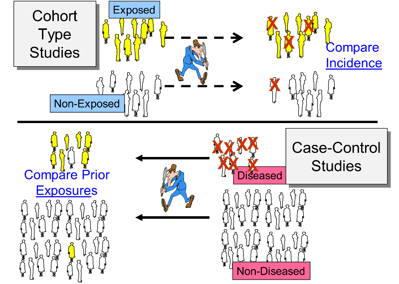
The cohort study design identifies a people exposed to a particular factor and a comparison group that was not exposed to that factor and measures and compares the incidence of disease in the two groups. A higher incidence of disease in the exposed group suggests an association between that factor and the disease outcome. This study design is generally a good choice when dealing with an outbreak in a relatively small, well-defined source population, particularly if the disease being studied was fairly frequent.
The case-control design uses a different sampling strategy in which the investigators identify a group of individuals who had developed the disease (the cases) and a comparison of individuals who did not have the disease of interest. The cases and controls are then compared with respect to the frequency of one or more past exposures. If the cases have a substantially higher odds of exposure to a particular factor compared to the control subjects, it suggests an association. This strategy is a better choice when the source population is large and ill-defined, and it is particularly useful when the disease outcome was uncommon. Examples of two real outbreaks will be used to illustrate these differences in sampling strategy.
A community in Massachusetts experienced an outbreak of Salmonellosis. Health officials noted that an unusually large number of cases had been reported during a span of several days. The table below summarizes some of the salient facts about Salmonella infections. Descriptive epidemiology was conducted, and hypothesis-generating interviews indicated that all of the disease people had attended a parent-teacher luncheon at a local school. In fact, it was a potluck luncheon, and the attendees each brought a dish that they had either prepared at home or purchased. The descriptive epidemiology convincingly indicated that the outbreak originated at the luncheon, but which specific dish was responsible? The investigators needed to establish which dish was responsible in order to clearly establish the source and to ensure that appropriate control measures were undertaken.
|
Salmonella Incubation period: 1-3 days
Symptoms: Diarrhea, fever, abdominal cramps, vomiting. S. Typhi and S. Paratyphi produce typhoid with insidious onset characterized by fever, headache, constipation, malaise, chills, myalgia; diarrhea is uncommon and vomiting is usually not severe.
Duration: 4-7 days
Sources: Contaminated eggs, poultry, unpasteurized milk or juice, cheese, contaminated raw fruits and vegetables (alfalfa sprouts, melons). S. Typhi epidemics are often related to fecal contamination of water supplies or street vended food. Other sources include pet rodents (hamsters, mice, and rats, or their bedding) and reptiles and amphibians (e.g., turtles, frogs, snakes, lizards, iguanas, etc.)
Laboratory Confirmation: Stool cultures
|
The source population was obviously the attendees of the luncheon, and 58% of the attendees had developed symptoms consistent with the case definition. Of these, 45 attendees agreed to complete a questionnaire regarding the foods that they had eaten at the luncheon. Since they had a relatively small, discrete cohort and a fairly high incidence of disease, a cohort design was a logical choice. For each dish served at the luncheon the investigators compared the incidence of Salmonellosis between those who ate a particular dish (the exposed group) and those who had not eaten that dish (the non-exposed comparison group). For each dish they constructed a contingency table to summarize the result from the survey. For example, the table below summarizes the findings from the survey regarding the incidence of disease in those who ate the cheese appetizer compared to those who did not eat it.

These results indicate that 23 attendees recalled eating the cheese appetizer, and 16 of them subsequently developed Salmonellosis, i.e., an incidence of 70%. There were 22 attendees who did not recall eating the cheese appetizer, and 9 or these developed symptoms of Salmonellosis, for an incidence of 41%.
When comparing the incidence of disease in an exposed group and an unexposed group, the magnitude of association is often summarized by computing a risk ratio, as follows.
Risk Ratio = (Incidence in the exposed group) / (Incidence in the unexposed group)
Therefore, for the Salmonella outbreak:
Risk Ratio = (16/23)/(9/22) = 0.70/0.41 = 1.70
This provides a means of estimating the magnitude of association between eating the cheese appetizer and risk of getting Salmonellosis. In order to complete the analysis, the investigators performed these computations for each of the dishes served at the luncheon. The table below summarizes all of the findings.
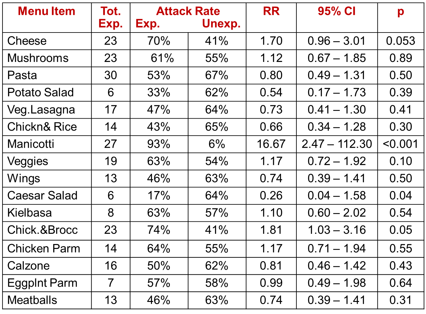
If there were no association between a particular exposure and risk of disease, then we would expect a risk ratio = 1.0. However, the overall sample was very small, and some of the dishes had very few takers, such as the potato salad. It is not surprising then that the risk ratios (column "RR") vary above and below a value of 1 as a result of random error (i.e., sampling error). One can assess the extent of random error by computing a 95% confidence interval for each estimated risk ratio (see the next to last column), and we can also compute a "p" value, as shown in the last column. A common interpretation of a 95% confidence interval for a risk ratio is that it is the range within which the true RR is likely to fall with 95% confidence. Conversely, the true value is unlikely to lie outside this range. The confidence interval also provides a measure of the precision of the estimated risk ratio. The p value is the probability of observing a difference between the exposed and unexposed groups this larger or larger if the groups truly didn't differ. The last three columns, then, help us put all of this into perspective. Most of the risk ratios (RR) are somewhat above or below a value of 1.0, which would indicate no difference. However, the risk ratio for exposure to manicotti was 16.67, suggesting that those who ate the manicotti had almost 17 times the risk of developing Salmonellosis. The 95% confidence interval for manicotti was very wide, but the lower limit of the interval was 2.47, suggesting that it is unlikely that the risk was less than 2.5-fold. Finally, the p value was less than 0.001, which indicates a very low probability that the difference was the result of random error. It would, therefore, be reasonable to conclude that the manicotti was the source of the Salmonella outbreak.
For more information about cohort studies, risk ratios, confidence intervals, and p values, please consult the following modules:
The Salmonella outbreak above occurred in a small, well-defined cohort, and the overall attack rate was 58%. A cohort study design works well in these circumstances. However, in most outbreaks the population is not well defined, and cohort studies are not feasible. A good example of this is an actual outbreak of hepatitis A that occurred in Marshfield, MA in 2004.
|
Excerpts from introduction of the report by the Massachusetts Department of Health
|
Within a short period of time 20 cases of hepatitis A were identified in the Marshfield area. The epidemic curve suggested a point source epidemic, and the spot map showed the cases to be spread across the entire South Shore of Massachusetts, although the pattern suggested a focus near Marshfield. Hypothesis-generating interviews resulted in five food establishments that were candidate sources. Moreover, the disease was rare, so that even if they interviewed a sample of patrons at each of the restaurants, it is most likely that few, if any would have had recent hepatitis, even from the responsible restaurant.
In a situation like this a case-control design is a much more efficient option. The investigators identified as many cases as possible (19 agreed to answer the questionnaire), and they selected a sample of 38 non-diseased people as a comparison group (the controls). In this case, the "controls" were non-diseased people who were matched to the cases with respect to age, gender, and neighborhood of residence. Investigators then ascertained the prior exposures of subjects in each group, focusing on food establishments and other possibly relevant exposures they had had during the past two months.
When using a case-control strategy for sampling, it is not possible to calculate the incidence (attack rate) in exposed and non-exposed subjects, because the denominators of the exposure groups are unknown. However, one can calculate the odds of disease in exposed and non-exposed subjects, and these can be expressed as an odds ratio, which is a good approximation of a risk ratio in a situation like this, i.e., when the outcome is rare. An odds ratio can be computed for each of the possible sources. Consider the following example:
| Cases | Controls | |
| Ate at Papa Gino's | 10 | 19 |
| Did not eat at Papa Gino's | 9 | 19 |
| 19 | 38 |
Given these hypothetical results, the odds that someone who ate a Papa Gino's was a case were 10/19, while the odds that someone not exposed to Papa Gino's became a case were 9/19. These odds are quite similar, and the odds ratio is close to 1.0. The odds ratio can be interpreted the same way as a risk ratio.
Odds Ratio = (10/19) / (9/19) = 1.1
This certainly provides no compelling evidence to suggest an association with Papa Gino's, but, as we did with the risk ratio, we could compute a 95% confidence interval for the odds ratio, and we could also compute a p value. In this case the 95% confidence interval is 0.37 to 3.35, and p= 0.85.
In contrast, consider the findings for Ron's Grill:
|
|
Cases |
Controls |
|
Ate at Ron's Grill |
18 |
7 |
|
Did not eat at Ron's |
1 |
29 |
|
|
19 |
38 |
For Ron's Grill the odds ratio would be computed as follows:
Odds Ratio = (18/7) / (1/29) = 75
This suggests that patrons of Ron's Grill had 75 times the risk of being a case compared to those who did not eat at Ron's. The other three restaurants that had been suspects had odds ratios that were close to 1.0. This certainly provides strong evidence that a Ron's Grill was the source of the outbreak, and further investigation confirmed that one of the food handlers at Ron's had recently had a subclinical case of hepatitis A.
In case-control studies, one of the most difficult decisions is how to select the the controls. Ideally they should be non-diseased people who come from the same source population as the cases, and, aside from their outcome status, they should be comparable to the cases in order to avoid selection bias. Note that in the Marshfield case-control study the controls were selected in a way to ensure that they were comparable with respect to age and gender and lived in similar neighborhoods.
For more information about the conduct and analysis of case-control studies, please see the online modules on:
For more information on developing questionnaires for outbreak studies, see:
If analytical studies do not confirm any of the hypotheses generated by descriptive epidemiology, then you need to go back to the descriptive epidemiology and consider other sources and routes of transmission.
In addition, even if analytical studies establish the source, it may be necessary to pursue the investigation in order to refine your understanding of the source. For example, in the Salmonella outbreak described on page 7 it was clear that the manicotti dish was responsible, but what was the specific source? Was the manicotti prepared at home? Was it purchased? What ingredient was responsible for contaminating the manicotti? Was it the eggs used in preparation of the pasta? Was it the cheese?
This step is listed toward the end, but, you obviously want to initiate prevention measures as soon as possible if you have identified the source, even if you haven't worked out all of the details.
When the investigation is concluded, it is important to communicate your findings to the local health authorities and to those responsible for implementing control and prevention measures. The communications usually require both oral and written reports. The written report should follow standard scientific guidelines, and it should include an introduction, background, methods, results, discussion, and recommendations.