


Confidence Interval for Two Independent Samples, Continuous Outcome
There are many situations where it is of interest to compare two groups with respect to their mean scores on a continuous outcome. For example, we might be interested in comparing mean systolic blood pressure in men and women, or perhaps compare body mass index (BMI) in smokers and non-smokers. Both of these situations involve comparisons between two independent groups , meaning that there are different people in the groups being compared.
We could begin by computing the sample sizes (n1 and n2), means ( and
and  ), and standard deviations (s1 and s2) in each sample.
In the two independent samples application with a continuous outcome, the parameter of interest is the difference in population means, μ1 - μ2. The point estimate for the difference in population means is the difference in sample means:

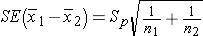
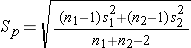
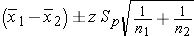
The confidence interval will be computed using either the Z or t distribution for the selected confidence level and the standard error of the point estimate. The use of Z or t again depends on whether the sample sizes are large (n1 > 30 and n2 > 30) or small. The standard error of the point estimate will incorporate the variability in the outcome of interest in each of the comparison groups. If we assume equal variances between groups, we can pool the information on variability (sample variances) to generate an estimate of the population variability. Therefore, the standard error (SE) of the difference in sample means is the pooled estimate of the common standard deviation (Sp) (assuming that the variances in the populations are similar) computed as the weighted average of the standard deviations in the samples, i.e.:
and the pooled estimate of the common standard deviation is
Computing the Confidence Interval for a Difference Between Two Means
If the sample sizes are larger, that is both n1 and n2 are greater than 30, then one uses the z-table.
If either sample size is less than 30, then the t-table is used.
- If n1 > 30 and n2 > 30, we can use the z-table:
Use Z table for standard normal distribution
- If n1 < 30 or n2 < 30, use the t-table:\
Use the t-table with degrees of freedom = n1+n2-2
For both large and small samples Sp is the pooled estimate of the common standard deviation (assuming that the variances in the populations are similar) computed as the weighted average of the standard deviations in the samples.
These formulas assume equal variability in the two populations (i.e., the population variances are equal, or σ12= σ22), meaning that the outcome is equally variable in each of the comparison populations. For analysis, we have samples from each of the comparison populations, and if the sample variances are similar, then the assumption about variability in the populations is reasonable. As a guideline, if the ratio of the sample variances, s12/s22 is between 0.5 and 2 (i.e., if one variance is no more than double the other), then the formulas in the table above are appropriate. If not, then alternative formulas must be used to account for the heterogeneity in variances.3,4
Large Sample Example:
The table below summarizes data n=3539 participants attending the 7th examination of the Offspring cohort in the Framingham Heart Study.
|
|
Men |
Women |
||||
|
Characteristic |
N |
|
s |
n |
|
s |
|
Systolic Blood Pressure |
1,623 |
128.2 |
17.5 |
1,911 |
126.5 |
20.1 |
|
Diastolic Blood Pressure |
1,622 |
75.6 |
9.8 |
1,910 |
72.6 |
9.7 |
|
Total Serum Cholesterol |
1,544 |
192.4 |
35.2 |
1,766 |
207.1 |
36.7 |
|
Weight |
1,612 |
194.0 |
33.8 |
1,894 |
157.7 |
34.6 |
|
Height |
1,545 |
68.9 |
2.7 |
1,781 |
63.4 |
2.5 |
|
Body Mass Index |
1,545 |
28.8 |
4.6 |
1,781 |
27.6 |
5.9 |

Suppose we want to calculate the difference in mean systolic blood pressures between men and women, and we also want the 95% confidence interval for the difference in means. The sample is large (> 30 for both men and women), so we can use the confidence interval formula with Z. Next, we will check the assumption of equality of population variances. The ratio of the sample variances is 17.52/20.12 = 0.76, which falls between 0.5 and 2, suggesting that the assumption of equality of population variances is reasonable.
First, we need to compute Sp, the pooled estimate of the common standard deviation.
Substituting we get
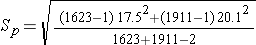
which simplifies to
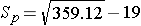
Notice that for this example Sp, the pooled estimate of the common standard deviation, is 19, and this falls in between the standard deviations in the comparison groups (i.e., 17.5 and 20.1). Next we substitute the Z score for 95% confidence, Sp=19, the sample means, and the sample sizes into the equation for the confidence interval.
Substituting
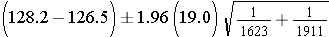
which simplifies to
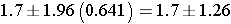
Therefore, the confidence interval is (0.44, 2.96)
Interpretation: With 95% confidence the difference in mean systolic blood pressures between men and women is between 0.44 and 2.96 units. Our best estimate of the difference, the point estimate, is 1.7 units. The standard error of the difference is 0.641, and the margin of error is 1.26 units. Note that when we generate estimates for a population parameter in a single sample (e.g., the mean [μ]) or population proportion [p]) the resulting confidence interval provides a range of likely values for that parameter. In contrast, when comparing two independent samples in this fashion the confidence interval provides a range of values for the difference. In this example, we estimate that the difference in mean systolic blood pressures is between 0.44 and 2.96 units with men having the higher values. In this example, we arbitrarily designated the men as group 1 and women as group 2. Had we designated the groups the other way (i.e., women as group 1 and men as group 2), the confidence interval would have been -2.96 to -0.44, suggesting that women have lower systolic blood pressures (anywhere from 0.44 to 2.96 units lower than men).
The table below summarizes differences between men and women with respect to the characteristics listed in the first column. The second and third columns show the means and standard deviations for men and women respectively. The fourth column shows the differences between males and females and the 95% confidence intervals for the differences.
|
|
Men |
Women |
Difference |
|
Characteristic |
Mean (s) |
Mean (s) |
95% CI |
|
Systolic Blood Pressure |
128.2 (17.5) |
126.5 (20.1) |
(0.44, 2.96) |
|
Diastolic Blood Pressure |
75.6 (9.8) |
72.6 (9.7) |
(2.38, 3.67) |
|
Total Serum Cholesterol |
192.4 (35.2) |
207.1 (36.7) |
(-17.16, -12.24) |
|
Weight |
194.0 (33.8) |
157.7 (34.6) |
(33.98, 38.53) |
|
Height |
68.9 (2.7) |
63.4 (2.5) |
(5.31, 5.66) |
|
Body Mass Index |
28.8 (4.6) |
27.6 (5.9) |
(0.76, 1.48) |
Notice that the 95% confidence interval for the difference in mean total cholesterol levels between men and women is -17.16 to -12.24. Men have lower mean total cholesterol levels than women; anywhere from 12.24 to 17.16 units lower. The men have higher mean values on each of the other characteristics considered (indicated by the positive confidence intervals).
The confidence interval for the difference in means provides an estimate of the absolute difference in means of the outcome variable of interest between the comparison groups. It is often of interest to make a judgment as to whether there is a statistically meaningful difference between comparison groups. This judgment is based on whether the observed difference is beyond what one would expect by chance.
The confidence intervals for the difference in means provide a range of likely values for (μ1-μ2). It is important to note that all values in the confidence interval are equally likely estimates of the true value of (μ1-μ2). If there is no difference between the population means, then the difference will be zero (i.e., (μ1-μ2).= 0). Zero is the null value of the parameter (in this case the difference in means). If a 95% confidence interval includes the null value, then there is no statistically meaningful or statistically significant difference between the groups. If the confidence interval does not include the null value, then we conclude that there is a statistically significant difference between the groups. For each of the characteristics in the table above there is a statistically significant difference in means between men and women, because none of the confidence intervals include the null value, zero. Note, however, that some of the means are not very different between men and women (e.g., systolic and diastolic blood pressure), yet the 95% confidence intervals do not include zero. This means that there is a small, but statistically meaningful difference in the means. When there are small differences between groups, it may be possible to demonstrate that the differences are statistically significant if the sample size is sufficiently large, as it is in this example.
Small Sample Example:
We previously considered a subsample of n=10 participants attending the 7th examination of the Offspring cohort in the Framingham Heart Study. The following table contains descriptive statistics on the same continuous characteristics in the subsample stratified by sex.
|
|
Men |
Women |
||||
|
Characteristic |
n |
Sample Mean |
s |
n |
Sample Mean |
s |
|
Systolic Blood Pressure |
6 |
117.5 |
9.7 |
4 |
126.8 |
12.0 |
|
Diastolic Blood Pressure |
6 |
72.5 |
7.1 |
4 |
69.5 |
8.1 |
|
Total Serum Cholesterol |
6 |
193.8 |
30.2 |
4 |
215.0 |
48.8 |
|
Weight |
6 |
196.9 |
26.9 |
4 |
146.0 |
7.2 |
|
Height |
6 |
70.2 |
1.0 |
4 |
62.6 |
2.3 |
|
Body Mass Index |
6 |
28.0 |
3.6 |
4 |
26.2 |
2.0 |
Suppose we wish to construct a 95% confidence interval for the difference in mean systolic blood pressures between men and women using these data. We will again arbitrarily designate men group 1 and women group 2. Since the sample sizes are small (i.e., n1< 30 and n2< 30), the confidence interval formula with t is appropriate. However,we will first check whether the assumption of equality of population variances is reasonable. The ratio of the sample variances is 9.72/12.02 = 0.65, which falls between 0.5 and 2, suggesting that the assumption of equality of population variances is reasonable. The solution is shown below.
First, we compute Sp, the pooled estimate of the common standard deviation:
Substituting:
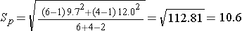
Note that again the pooled estimate of the common standard deviation, Sp, falls in between the standard deviations in the comparison groups (i.e., 9.7 and 12.0). The degrees of freedom (df) = n1+n2-2 = 6+4-2 = 8. From the t-Table t=2.306. The 95% confidence interval for the difference in mean systolic blood pressures is:
Substituting:

Then simplifying further:
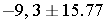
So, the 95% confidence interval for the difference is (-25.07, 6.47)
Interpretation: Our best estimate of the difference, the point estimate, is -9.3 units. The standard error of the difference is 6.84 units and the margin of error is 15.77 units. We are 95% confident that the difference in mean systolic blood pressures between men and women is between -25.07 and 6.47 units. In this sample, the men have lower mean systolic blood pressures than women by 9.3 units. Based on this interval, we also conclude that there is no statistically significant difference in mean systolic blood pressures between men and women, because the 95% confidence interval includes the null value, zero. Again, the confidence interval is a range of likely values for the difference in means. Since the interval contains zero (no difference), we do not have sufficient evidence to conclude that there is a difference. Note also that this 95% confidence interval for the difference in mean blood pressures is much wider here than the one based on the full sample derived in the previous example, because the very small sample size produces a very imprecise estimate of the difference in mean systolic blood pressures.