

Introduction to Correlation and Regression Analysis
In this section we will first discuss correlation analysis, which is used to quantify the association between two continuous variables (e.g., between an independent and a dependent variable or between two independent variables). Regression analysis is a related technique to assess the relationship between an outcome variable and one or more risk factors or confounding variables. The outcome variable is also called the response or dependent variable and the risk factors and confounders are called the predictors, or explanatory or independent variables. In regression analysis, the dependent variable is denoted "y" and the independent variables are denoted by "x".
[NOTE: The term "predictor" can be misleading if it is interpreted as the ability to predict even beyond the limits of the data. Also, the term "explanatory variable" might give an impression of a causal effect in a situation in which inferences should be limited to identifying associations. The terms "independent" and "dependent" variable are less subject to these interpretations as they do not strongly imply cause and effect.
Correlation Analysis
In correlation analysis, we estimate a sample correlation coefficient, more specifically the Pearson Product Moment correlation coefficient. The sample correlation coefficient, denoted r,
ranges between -1 and +1 and quantifies the direction and strength of the linear association between the two variables. The correlation between two variables can be positive (i.e., higher levels of one variable are associated with higher levels of the other) or negative (i.e., higher levels of one variable are associated with lower levels of the other).
The sign of the correlation coefficient indicates the direction of the association. The magnitude of the correlation coefficient indicates the strength of the association.
For example, a correlation of r = 0.9 suggests a strong, positive association between two variables, whereas a correlation of r = -0.2 suggest a weak, negative association. A correlation close to zero suggests no linear association between two continuous variables.
LISA: [I find this description confusing. You say that the correlation coefficient is a measure of the "strength of association", but if you think about it, isn't the slope a better measure of association? We use risk ratios and odds ratios to quantify the strength of association, i.e., when an exposure is present it has how many times more likely the outcome is. The analogous quantity in correlation is the slope, i.e., for a given increment in the independent variable, how many times is the dependent variable going to increase? And "r" (or perhaps better R-squared) is a measure of how much of the variability in the dependent variable can be accounted for by differences in the independent variable. The analogous measure for a dichotomous variable and a dichotomous outcome would be the attributable proportion, i.e., the proportion of Y that can be attributed to the presence of the exposure.]
It is important to note that there may be a non-linear association between two continuous variables, but computation of a correlation coefficient does not detect this. Therefore, it is always important to evaluate the data carefully before computing a correlation coefficient. Graphical displays are particularly useful to explore associations between variables.
The figure below shows four hypothetical scenarios in which one continuous variable is plotted along the X-axis and the other along the Y-axis.
|
|
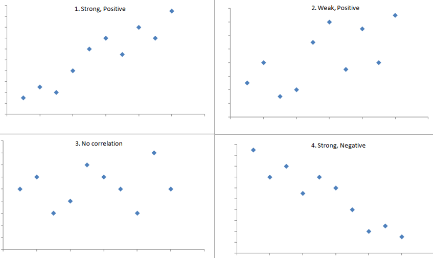
- Scenario 1 depicts a strong positive association (r=0.9), similar to what we might see for the correlation between infant birth weight and birth length.
- Scenario 2 depicts a weaker association (r=0,2) that we might expect to see between age and body mass index (which tends to increase with age).
- Scenario 3 might depict the lack of association (r approximately 0) between the extent of media exposure in adolescence and age at which adolescents initiate sexual activity.
- Scenario 4 might depict the strong negative association (r= -0.9) generally observed between the number of hours of aerobic exercise per week and percent body fat.
Example - Correlation of Gestational Age and Birth Weight
A small study is conducted involving 17 infants to investigate the association between gestational age at birth, measured in weeks, and birth weight, measured in grams.
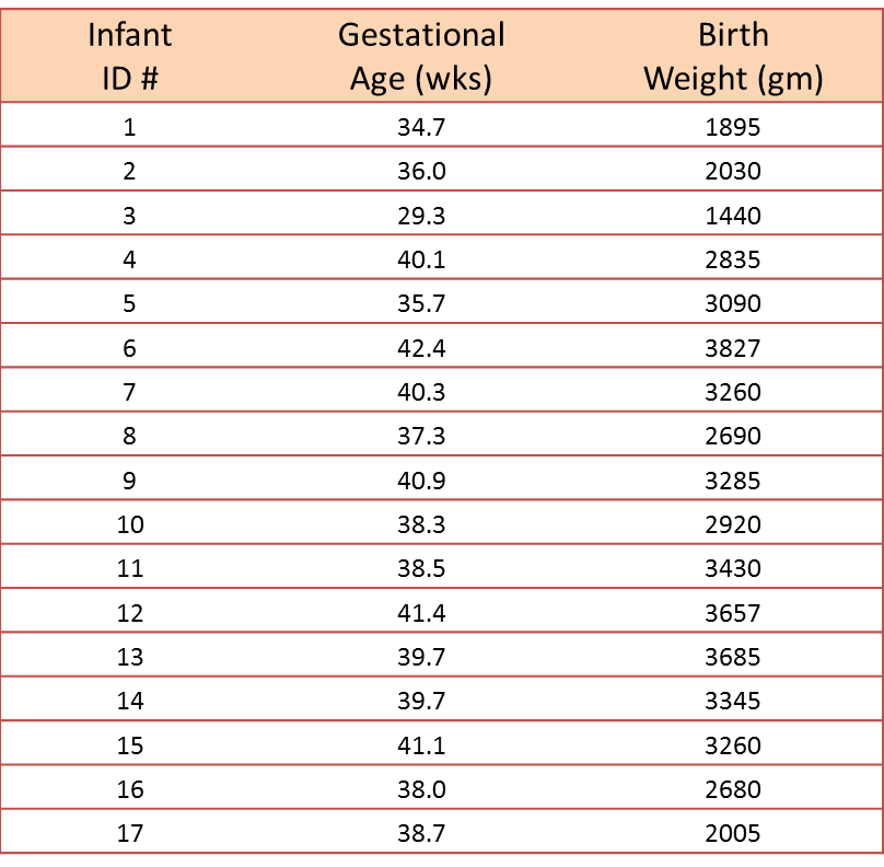
We wish to estimate the association between gestational age and infant birth weight. In this example, birth weight is the dependent variable and gestational age is the independent variable. Thus y=birth weight and x=gestational age. The data are displayed in a scatter diagram in the figure below.
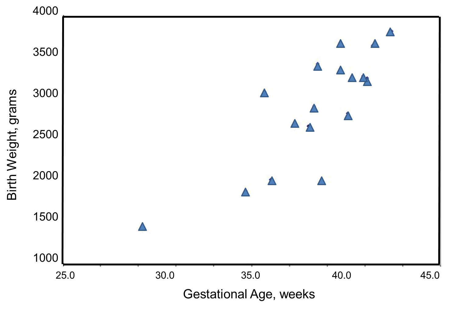
Each point represents an (x,y) pair (in this case the gestational age, measured in weeks, and the birth weight, measured in grams). Note that the independent variable is on the horizontal axis (or X-axis), and the dependent variable is on the vertical axis (or Y-axis). The scatter plot shows a positive or direct association between gestational age and birth weight. Infants with shorter gestational ages are more likely to be born with lower weights and infants with longer gestational ages are more likely to be born with higher weights.
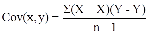
The formula for the sample correlation coefficient is
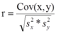
where Cov(x,y) is the covariance of x and y defined as
![]()
![]() are the sample variances of x and y, defined as
are the sample variances of x and y, defined as
![]()
The variances of x and y measure the variability of the x scores and y scores around their respective sample means (
![]() , considered separately). The covariance measures the variability of the (x,y) pairs around the mean of x and mean of y, considered simultaneously.
, considered separately). The covariance measures the variability of the (x,y) pairs around the mean of x and mean of y, considered simultaneously.
To compute the sample correlation coefficient, we need to compute the variance of gestational age, the variance of birth weight and also the covariance of gestational age and birth weight.
We first summarize the gestational age data. The mean gestational age is:
![]()
To compute the variance of gestational age, we need to sum the squared deviations (or differences) between each observed gestational age and the mean gestational age. The computations are summarized below.
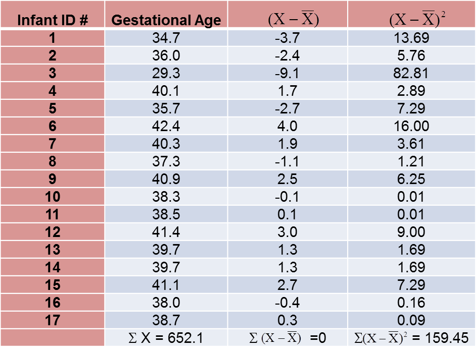
The variance of gestational age is:
![]()
Next, we summarize the birth weight data. The mean birth weight is:
![]()
The variance of birth weight is computed just as we did for gestational age as shown in the table below.
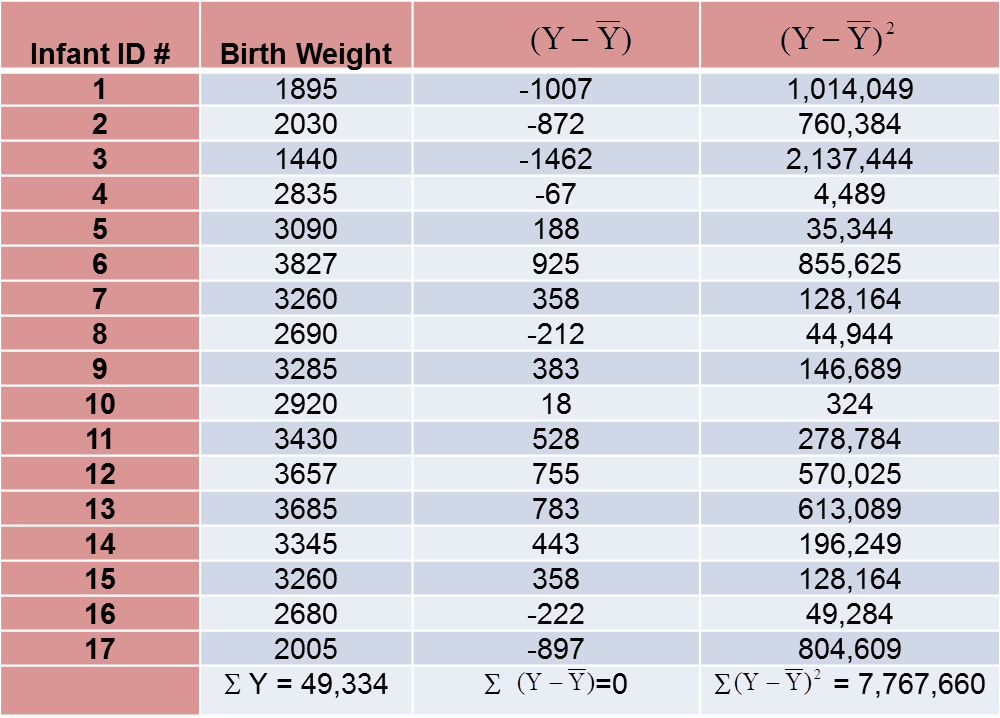
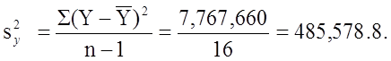
The variance of birth weight is:
Next we compute the covariance,
To compute the covariance of gestational age and birth weight, we need to multiply the deviation from the mean gestational age by the deviation from the mean birth weight for each participant (i.e.,
![]()
The computations are summarized below. Notice that we simply copy the deviations from the mean gestational age and birth weight from the two tables above into the table below and multiply.
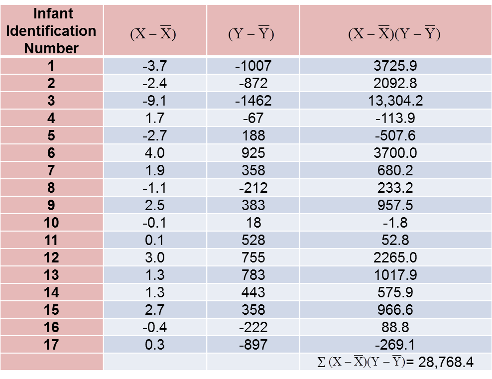
The covariance of gestational age and birth weight is:
![]()
We now compute the sample correlation coefficient:
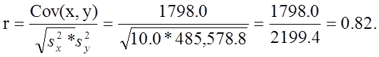
Not surprisingly, the sample correlation coefficient indicates a strong positive correlation.
As we noted, sample correlation coefficients range from -1 to +1. In practice, meaningful correlations (i.e., correlations that are clinically or practically important) can be as small as 0.4 (or -0.4) for positive (or negative) associations. There are also statistical tests to determine whether an observed correlation is statistically significant or not (i.e., statistically significantly different from zero). Procedures to test whether an observed sample correlation is suggestive of a statistically significant correlation are described in detail in Kleinbaum, Kupper and Muller.1