

Regression Analysis
Regression analysis is a widely used technique which is useful for evaluating multiple independent variables. As a result, it is particularly useful for assess and adjusting for confounding. It can also be used to assess the presence of effect modification. Interested readers should see Kleinbaum, Kupper and Muller for more details on regression analysis and its many applications.1
Simple Linear Regression
Suppose we want to assess the association between total cholesterol and body mass index (BMI) in which total cholesterol is the dependent variable, and BMI is the independent variable. In regression analysis, the dependent variable is denoted Y and the independent variable is denoted X. So, in this case, Y=total cholesterol and X=BMI.
When there is a single continuous dependent variable and a single independent variable, the analysis is called a simple linear regression analysis. This analysis assumes that there is a linear association between the two variables. (If a different relationship is hypothesized, such as a curvilinear or exponential relationship, alternative regression analyses are performed.)
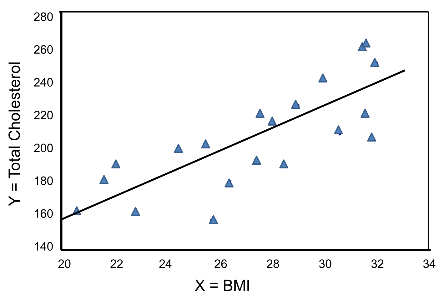
The figure below is a scatter diagram illustrating the relationship between BMI and total cholesterol. Each point represents the (X, Y) pair, in this case, BMI and the corresponding total cholesterol measured in each participant. Note that the independent variable is on the horizontal axis and the dependent variable on the vertical axis.
BMI and Total Cholesterol
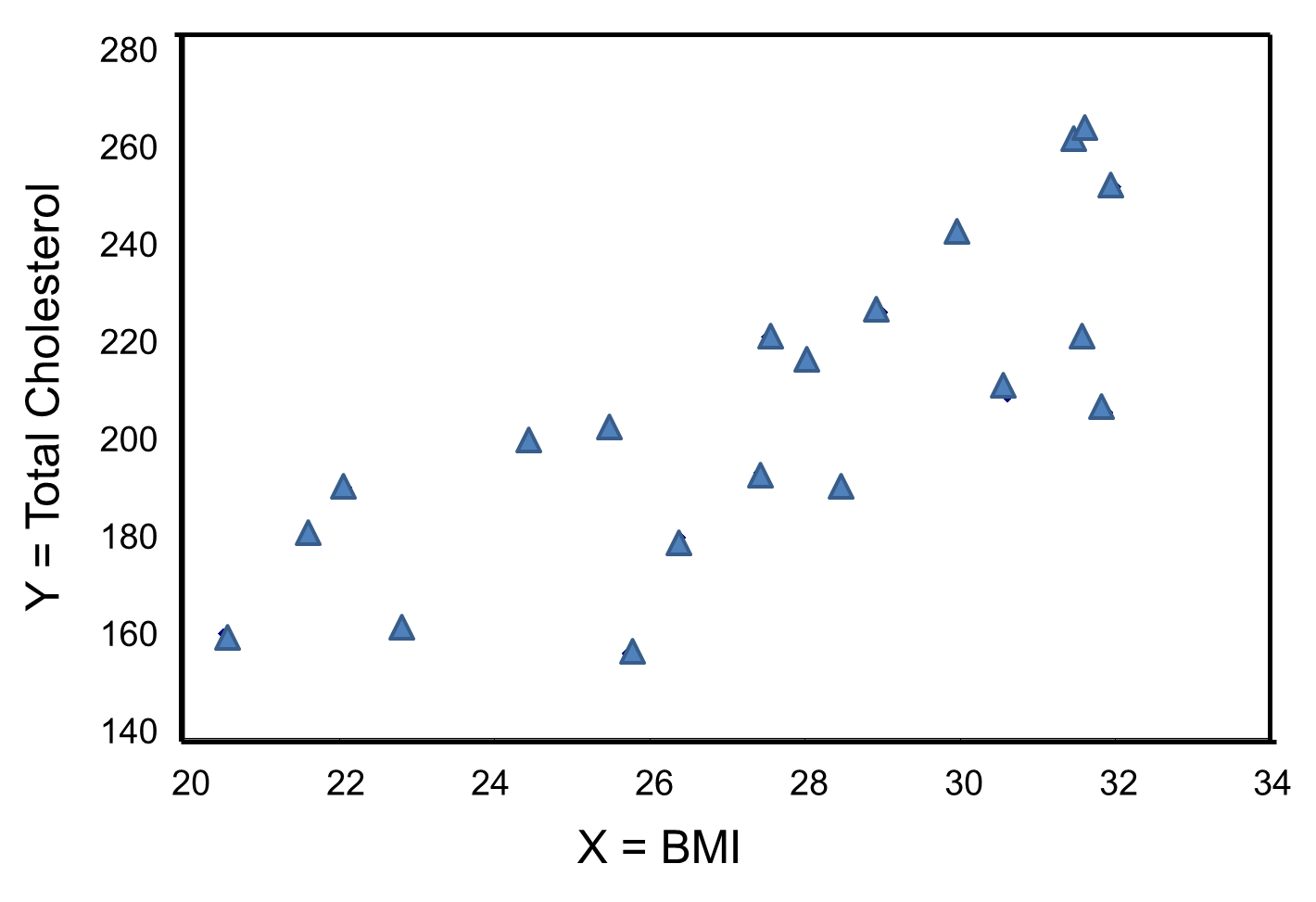
The graph shows that there is a positive or direct association between BMI and total cholesterol; participants with lower BMI are more likely to have lower total cholesterol levels and participants with higher BMI are more likely to have higher total cholesterol levels. In contrast, suppose we examine the association between BMI and HDL cholesterol.
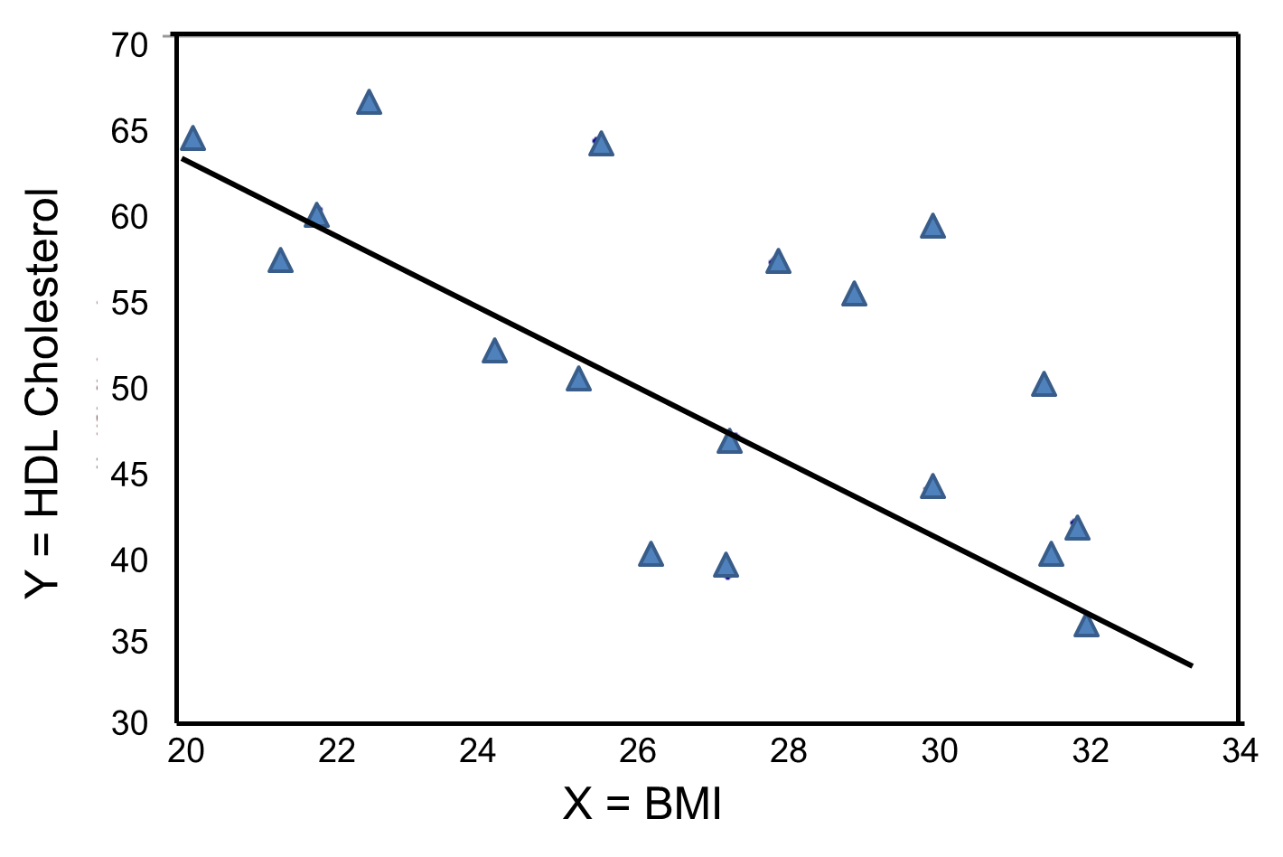
In contrast, the graph below depicts the relationship between BMI and HDL HDL cholesterol in the same sample of n=20 participants.
BMI and HDL Cholesterol
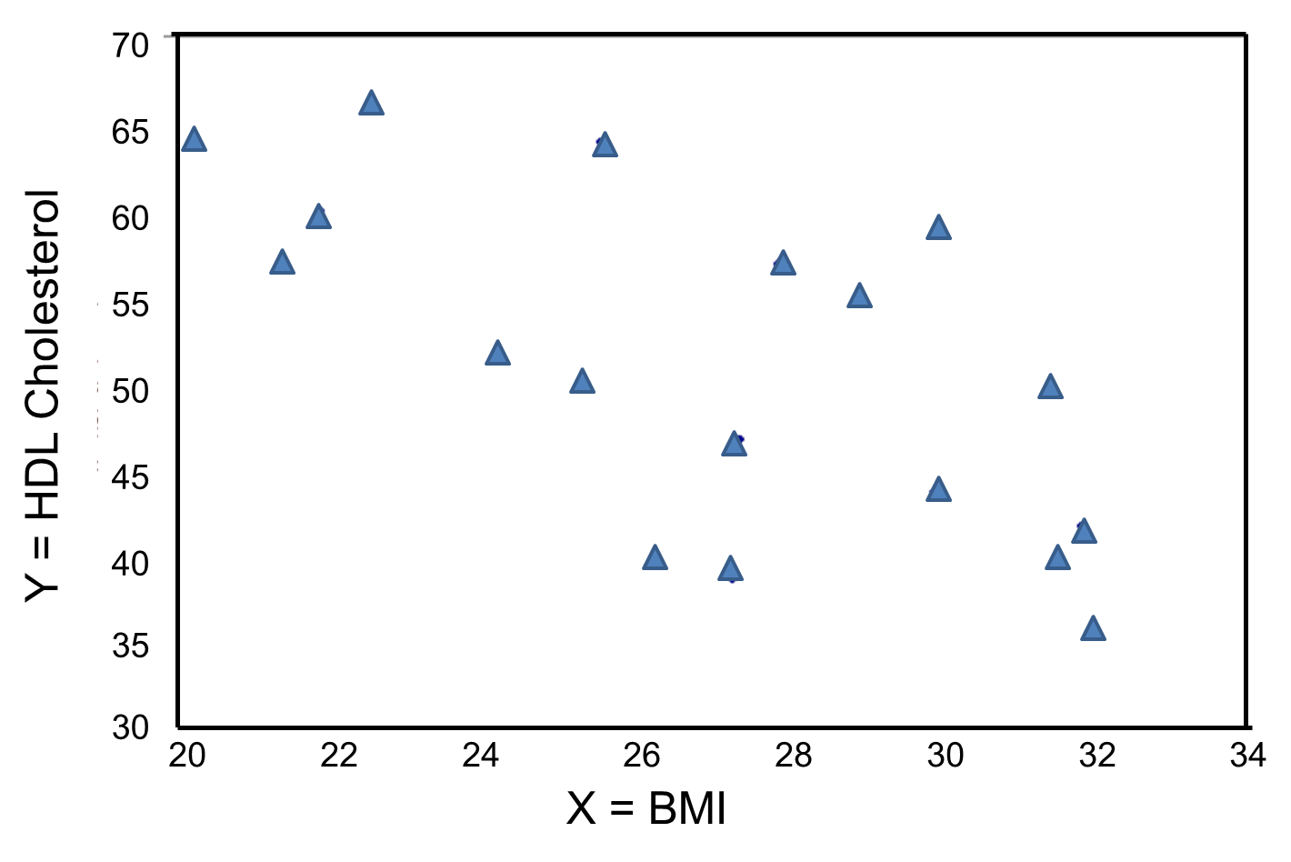
This graph shows a negative or inverse association between BMI and HDL cholesterol, i.e., those with lower BMI are more likely to have higher HDL cholesterol levels and those with higher BMI are more likely to have lower HDL cholesterol levels.
For either of these relationships we could use simple linear regression analysis to estimate the equation of the line that best describes the association between the independent variable and the dependent variable. The simple linear regression equation is as follows:
![]() , where
, where
![]() is the predicted or expected value of the outcome, X is the predictor , b0 is the estimated Y-intercept, and b1 is the estimated slope. The Y-intercept and slope are estimated from the sample data so as to minimize the sum of the squared differences between the observed and the predicted values of the outcome, i.e., the estimates minimize:
is the predicted or expected value of the outcome, X is the predictor , b0 is the estimated Y-intercept, and b1 is the estimated slope. The Y-intercept and slope are estimated from the sample data so as to minimize the sum of the squared differences between the observed and the predicted values of the outcome, i.e., the estimates minimize:
![]()
These differences between observed and predicted values of the outcome are called residuals. The estimates of the Y-intercept and slope minimize the sum of the squared residuals, and are called the least squares estimates.1
|
Residuals |
|---|
|
Conceptually, if the values of X provided a perfect prediction of Y then the sum of the squared differences between observed and predicted values of Y would be 0. That would mean that variability in Y could be completely explained by differences in X. However, if the differences between observed and predicted values are not 0, then we are unable to entirely account for differences in Y based on X, then there are residual errors in the prediction. The residual error could result from inaccurate measurements of X or Y, or there could be other variables besides X that affect the value of Y. |
Based on the observed data, the best estimate of a linear relationship will be obtained from an equation for the line that minimizes the differences between observed and predicted values of the outcome. The Y-intercept of this line is the value of the dependent variable (Y) when the independent variable (X) is zero. The slope of the line is the change in the dependent variable (Y) relative to a one unit change in the independent variable (X). The least squares estimates of the y-intercept and slope are computed as follows:
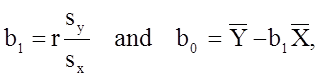
where
- r is the sample correlation coefficient,
- the sample means are
 and
and 
- and Sx and Sy are the standard deviations of the independent variable x and the dependent variable y, respectively.
BMI and Total Cholesterol
The least squares estimates of the regression coefficients, b 0 and b1, describing the relationship between BMI and total cholesterol are b0 = 28.07 and b1=6.49. These are computed as follows:

The estimate of the Y-intercept (b0 = 28.07) represents the estimated total cholesterol level when BMI is zero. Because a BMI of zero is meaningless, the Y-intercept is not informative. The estimate of the slope (b1 = 6.49) represents the change in total cholesterol relative to a one unit change in BMI. For example, if we compare two participants whose BMIs differ by 1 unit, we would expect their total cholesterols to differ by approximately 6.49 units (with the person with the higher BMI having the higher total cholesterol).
The equation of the regression line is as follows:
![]()
The graph below shows the estimated regression line superimposed on the scatter diagram.
The regression equation can be used to estimate a participant's total cholesterol as a function of his/her BMI. For example, suppose a participant has a BMI of 25. We would estimate their total cholesterol to be 28.07 + 6.49(25) = 190.32. The equation can also be used to estimate total cholesterol for other values of BMI. However, the equation should only be used to estimate cholesterol levels for persons whose BMIs are in the range of the data used to generate the regression equation. In our sample, BMI ranges from 20 to 32, thus the equation should only be used to generate estimates of total cholesterol for persons with BMI in that range.
There are statistical tests that can be performed to assess whether the estimated regression coefficients (b0 and b1) are statistically significantly different from zero. The test of most interest is usually H0: b1=0 versus H1: b1≠0, where b1 is the population slope. If the population slope is significantly different from zero, we conclude that there is a statistically significant association between the independent and dependent variables.
BMI and HDL Cholesterol
The least squares estimates of the regression coefficients, b0 and b1, describing the relationship between BMI and HDL cholesterol are as follows: b0 = 111.77 and b1 = -2.35. These are computed as follows:

Again, the Y-intercept in uninformative because a BMI of zero is meaningless. The estimate of the slope (b1 = -2.35) represents the change in HDL cholesterol relative to a one unit change in BMI. If we compare two participants whose BMIs differ by 1 unit, we would expect their HDL cholesterols to differ by approximately 2.35 units (with the person with the higher BMI having the lower HDL cholesterol. The figure below shows the regression line superimposed on the scatter diagram for BMI and HDL cholesterol.
Linear regression analysis rests on the assumption that the dependent variable is continuous and that the distribution of the dependent variable (Y) at each value of the independent variable (X) is approximately normally distributed. Note, however, that the independent variable can be continuous (e.g., BMI) or can be dichotomous (see below).
Comparing Mean HDL Levels With Regression Analysis
We previously considered data from a clinical trial that evaluated the efficacy of a new drug to increase HDL cholesterol (see page 4 of this module). We compared the mean HDL levels between treatment groups using a two independent samples t test. Note, however, that regression analysis can also be used to compare mean HDL levels between treatments.
HDL cholesterol is the continuous dependent variable and treatment (new drug versus placebo) is the independent variable. A simple linear regression equation is estimated as follows:
![]() where
where
![]() is the estimated HDL level and X is a dichotomous variable (also called an indicator variable, i.e., indicating whether the active treatment was given or not). In this example, X is coded as 1 for participants who received the new drug and as 0 for participants who received the placebo.
is the estimated HDL level and X is a dichotomous variable (also called an indicator variable, i.e., indicating whether the active treatment was given or not). In this example, X is coded as 1 for participants who received the new drug and as 0 for participants who received the placebo.
The estimate of the Y-intercept is b0=39.21. The Y-intercept is the value of Y (HDL cholesterol) when X is zero. In this example, X=0 indicates the placebo group. Thus, the Y-intercept is exactly equal to the mean HDL level in the placebo group. The slope is b1=0.95. The slope represents the change in Y (HDL cholesterol) relative to a one unit change in X. A one unit change in X represents a difference in treatment assignment (placebo versus new drug). The slope represents the difference in mean HDL levels between the treatment groups. Dichotomous (or indicator) variables are usually coded as 0 or 1, where 0 is assigned to participants who do not have a particular risk factor, exposure or characteristic and 1 is assigned to participants who have the particular risk factor, exposure or characteristic. In a later section we will present multiple logistic regression analysis which applies in situations where the outcome is dichotomous (e.g., incident CVD).
The Controversy Over Environmental Tobacco Smoke Exposure
There is convincing evidence that active smoking is a cause of lung cancer and heart disease. Many studies done in a wide variety of circumstances have consistently demonstrated a strong association and also indicate that the risk of lung cancer and cardiovascular disease (i.e.., heart attacks) increases in a dose-related way. These studies have led to the conclusion that active smoking is causally related to lung cancer and cardiovascular disease. Studies in active smokers have had the advantage that the lifetime exposure to tobacco smoke can be quantified with reasonable accuracy, since the unit dose is consistent (one cigarette) and the habitual nature of tobacco smoking makes it possible for most smokers to provide a reasonable estimate of their total lifetime exposure quantified in terms of cigarettes per day or packs per day. Frequently, average daily exposure (cigarettes or packs) is combined with duration of use in years in order to quantify exposure as "pack-years".
It has been much more difficult to establish whether environmental tobacco smoke (ETS) exposure is causally related to chronic diseases like heart disease and lung cancer, because the total lifetime exposure dosage is lower, and it is much more difficult to accurately estimate total lifetime exposure. In addition, quantifying these risks is also complicated because of confounding factors. For example, ETS exposure is usually classified based on parental or spousal smoking, but these studies are unable to quantify other environmental exposures to tobacco smoke, and inability to quantify and adjust for other environmental exposures such as air pollution makes it difficult to demonstrate an association even if one existed. As a result, there continues to be controversy over the risk imposed by environmental tobacco smoke (ETS). Some have gone so far as to claim that even very brief exposure to ETS can cause a myocardial infarction (heart attack), but a very large prospective cohort study by Estrom and Kabat was unable to demonstrate significant associations between exposure to spousal ETS and coronary heart disease, chronic obstructive pulmonary disease, or lung cancer. (It should be noted, however, that the report by Enstrom and Kabat has been widely criticized for methodologic problems, and these authors also had financial ties to the tobacco industry.)
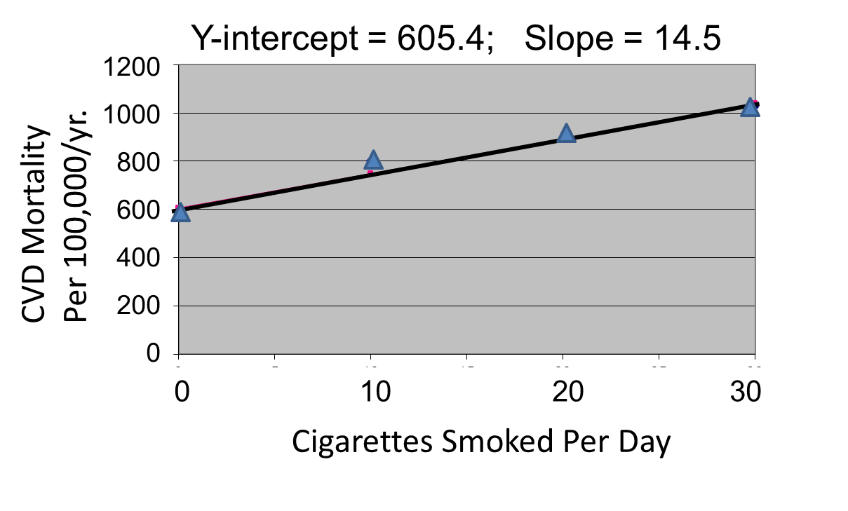
Correlation analysis provides a useful tool for thinking about this controversy. Consider data from the British Doctors Cohort. They reported the annual mortality for a variety of disease at four levels of cigarette smoking per day: Never smoked, 1-14/day, 15-24/day, and 25+/day. In order to perform a correlation analysis, I rounded the exposure levels to 0, 10, 20, and 30 respectively.
|
Cigarettes Smoked Per Day |
CVD Mortality/100,000 men/yr. |
Lung Cancer Mortality/100,000 men/yr. |
|---|---|---|
|
0 |
572 |
14 |
|
10 (actually 1-14) |
802 |
105 |
|
20 (actually 15-24) |
892 |
208 |
|
30 (actually >24) |
1025 |
355 |
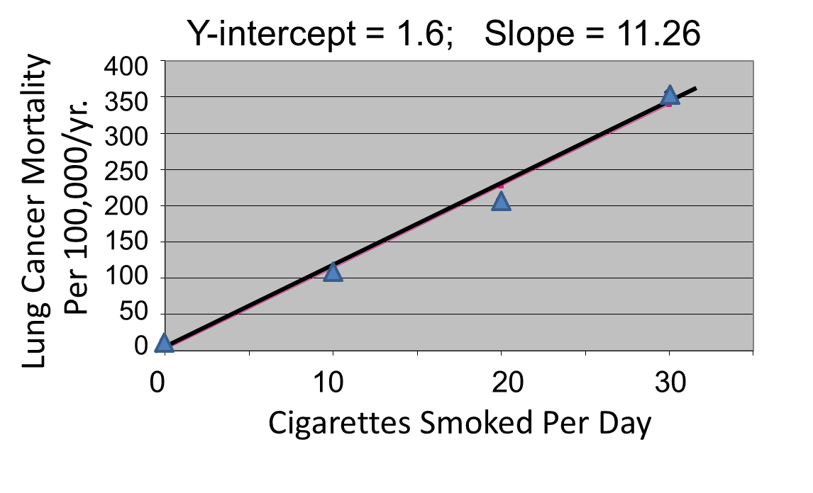
The figures below show the two estimated regression lines superimposed on the scatter diagram. The correlation with amount of smoking was strong for both CVD mortality (r= 0.98) and for lung cancer (r = 0.99). Note also that the Y-intercept is a meaningful number here; it represents the predicted annual death rate from these disease in individuals who never smoked. The Y-intercept for prediction of CVD is slightly higher than the observed rate in never smokers, while the Y-intercept for lung cancer is lower than the observed rate in never smokers.
The linearity of these relationships suggests that there is an incremental risk with each additional cigarette smoked per day, and the additional risk is estimated by the slopes. This perhaps helps us think about the consequences of ETS exposure. For example, the risk of lung cancer in never smokers is quite low, but there is a finite risk; various reports suggest a risk of 10-15 lung cancers/100,000 per year. If an individual who never smoked actively was exposed to the equivalent of one cigarette's smoke in the form of ETS, then the regression suggests that their risk would increase by 11.26 lung cancer deaths per 100,000 per year. However, the risk is clearly dose-related. Therefore, if a non-smoker was employed by a tavern with heavy levels of ETS, the risk might be substantially greater.
|
|
|
Finally, it should be noted that some findings suggest that the association between smoking and heart disease is non-linear at the very lowest exposure levels, meaning that non-smokers have a disproportionate increase in risk when exposed to ETS due to an increase in platelet aggregation.