


Comparing Survival Curves
We are often interested in assessing whether there are differences in survival (or cumulative incidence of event) among different groups of participants. For example, in a clinical trial with a survival outcome, we might be interested in comparing survival between participants receiving a new drug as compared to a placebo (or standard therapy). In an observational study, we might be interested in comparing survival between men and women, or between participants with and without a particular risk factor (e.g., hypertension or diabetes). There are several tests available to compare survival among independent groups.
The Log Rank Test
The log rank test is a popular test to test the null hypothesis of no difference in survival between two or more independent groups. The test compares the entire survival experience between groups and can be thought of as a test of whether the survival curves are identical (overlapping) or not. Survival curves are estimated for each group, considered separately, using the Kaplan-Meier method and compared statistically using the log rank test. It is important to note that there are several variations of the log rank test statistic that are implemented by various statistical computing packages (e.g., SAS, R 4,6). We present one version here that is linked closely to the chi-square test statistic and compares observed to expected numbers of events at each time point over the follow-up period.
Example:
A small clinical trial is run to compare two combination treatments in patients with advanced gastric cancer. Twenty participants with stage IV gastric cancer who consent to participate in the trial are randomly assigned to receive chemotherapy before surgery or chemotherapy after surgery. The primary outcome is death and participants are followed for up to 48 months (4 years) following enrollment into the trial. The experiences of participants in each arm of the trial are shown below.
|
Chemotherapy Before Surgery |
|
Chemotherapy After Surgery |
||
|---|---|---|---|---|
|
Month of Death |
Month of Last Contact |
|
Month of Death |
Month of Last Contact |
|
8 |
8 |
|
33 |
48 |
|
12 |
32 |
|
28 |
48 |
|
26 |
20 |
|
41 |
25 |
|
14 |
40 |
|
|
37 |
|
21 |
|
|
|
48 |
|
27 |
|
|
|
25 |
|
|
|
|
|
43 |
Six participants in the chemotherapy before surgery group die over the course of follow-up as compared to three participants in the chemotherapy after surgery group. Other participants in each group are followed for varying numbers of months, some to the end of the study at 48 months (in the chemotherapy after surgery group). Using the procedures outlined above, we first construct life tables for each treatment group using the Kaplan-Meier approach.
Life Table for Group Receiving Chemotherapy Before Surgery
|
Time, Months |
Number at Risk Nt |
Number of Deaths Dt |
Number Censored Ct |
Survival Probability
|
|---|---|---|---|---|
|
0 |
10 |
|
|
1 |
|
8 |
10 |
1 |
1 |
0.900 |
|
12 |
8 |
1 |
|
0.788 |
|
14 |
7 |
1 |
|
0.675 |
|
20 |
6 |
|
1 |
0.675 |
|
21 |
5 |
1 |
|
0.540 |
|
26 |
4 |
1 |
|
0.405 |
|
27 |
3 |
1 |
|
0.270 |
|
32 |
2 |
|
1 |
0.270 |
|
40 |
1 |
|
1 |
0.270 |
Life Table for Group Receiving Chemotherapy After Surgery
|
Time, Months |
Number at Risk Nt |
Number of Deaths Dt |
Number Censored Ct |
Survival Probability
|
|---|---|---|---|---|
|
0 |
10 |
|
|
1 |
|
25 |
10 |
|
2 |
1.000 |
|
28 |
8 |
1 |
|
0.875 |
|
33 |
7 |
1 |
|
0.750 |
|
37 |
6 |
|
1 |
0.750 |
|
41 |
5 |
1 |
|
0.600 |
|
43 |
4 |
|
1 |
0.600 |
|
48 |
3 |
|
3 |
0.600 |
The two survival curves are shown below.
Survival in Each Treatment Group
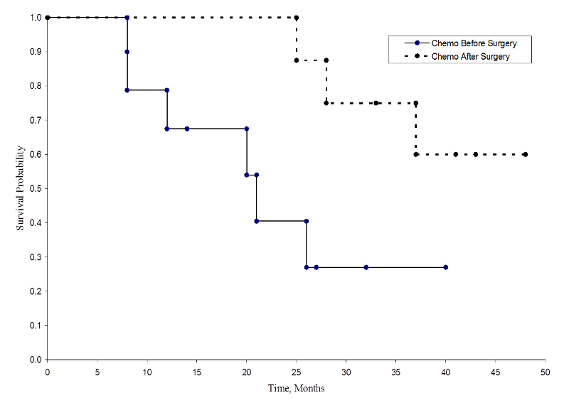
The survival probabilities for the chemotherapy after surgery group are higher than the survival probabilities for the chemotherapy before surgery group, suggesting a survival benefit. However, these survival curves are estimated from small samples. To compare survival between groups we can use the log rank test. The null hypothesis is that there is no difference in survival between the two groups or that there is no difference between the populations in the probability of death at any point. The log rank test is a non-parametric test and makes no assumptions about the survival distributions. In essence, the log rank test compares the observed number of events in each group to what would be expected if the null hypothesis were true (i.e., if the survival curves were identical).
H0: The two survival curves are identical (or S1t = S2t) versus H1: The two survival curves are not identical (or S1t ≠ S2t, at any time t) (α=0.05).
The log rank statistic is approximately distributed as a chi-square test statistic. There are several forms of the test statistic, and they vary in terms of how they are computed. We use the following:

where ΣOjt represents the sum of the observed number of events in the jth group over time (e.g., j=1,2) and ΣEjt represents the sum of the expected number of events in the jth group over time.
The sums of the observed and expected numbers of events are computed for each event time and summed for each comparison group. The log rank statistic has degrees of freedom equal to k-1, where k represents the number of comparison groups. In this example, k=2 so the test statistic has 1 degree of freedom.
To compute the test statistic we need the observed and expected number of events at each event time. The observed number of events are from the sample and the expected number of events are computed assuming that the null hypothesis is true (i.e., that the survival curves are identical).
To generate the expected numbers of events we organize the data into a life table with rows representing each event time, regardless of the group in which the event occurred. We also keep track of group assignment. We then estimate the proportion of events that occur at each time (Ot/Nt) using data from both groups combined under the assumption of no difference in survival (i.e., assuming the null hypothesis is true). We multiply these estimates by the number of participants at risk at that time in each of the comparison groups (N1t and N2t for groups 1 and 2 respectively).
Specifically, we compute for each event time t, the number at risk in each group, Njt (e.g., where j indicates the group, j=1, 2) and the number of events (deaths), Ojt ,in each group. The table below contains the information needed to conduct the log rank test to compare the survival curves above. Group 1 represents the chemotherapy before surgery group, and group 2 represents the chemotherapy after surgery group.
Data for Log Rank Test to Compare Survival Curves
|
Time, Months |
Number at Risk in Group 1
N1t |
Number at Risk in Group 2
N2t |
Number of Events (Deaths) in Group 1
O1t |
Number of Events (Deaths) in Group 2
O2t |
|---|---|---|---|---|
|
8 |
10 |
10 |
1 |
0 |
|
12 |
8 |
10 |
1 |
0 |
|
14 |
7 |
10 |
1 |
0 |
|
21 |
5 |
10 |
1 |
0 |
|
26 |
4 |
8 |
1 |
0 |
|
27 |
3 |
8 |
1 |
0 |
|
28 |
2 |
8 |
0 |
1 |
|
33 |
1 |
7 |
0 |
1 |
|
41 |
0 |
5 |
0 |
1 |
We next total the number at risk, Nt = N1t+N2t, at each event time and the number of observed events (deaths), Ot = O1t+O2t, at each event time. We then compute the expected number of events in each group. The expected number of events is computed at each event time as follows:
E1t = N1t*(Ot/Nt) for group 1 and E2t = N2t*(Ot/Nt) for group 2. The calculations are shown in the table below.
Expected Numbers of Events in Each Group
|
Time, Months |
Number at Risk in Group 1 N1t |
Number at Risk in Group 2 N2t |
Total Number at Risk Nt |
Number of Events in Group 1 O1t |
Number of Events in Group 2 O2t |
Total Number of Events Ot |
Expected Number of Events in Group 1 E1t = N1t*(Ot/Nt) |
Expected Number of Events in Group 2 E2t = N2t*(Ot/Nt) |
|---|---|---|---|---|---|---|---|---|
|
8 |
10 |
10 |
20 |
1 |
0 |
1 |
0.500 |
0.500 |
|
12 |
8 |
10 |
18 |
1 |
0 |
1 |
0.444 |
0.556 |
|
14 |
7 |
10 |
17 |
1 |
0 |
1 |
0.412 |
0.588 |
|
21 |
5 |
10 |
15 |
1 |
0 |
1 |
0.333 |
0.667 |
|
26 |
4 |
8 |
12 |
1 |
0 |
1 |
0.333 |
0.667 |
|
27 |
3 |
8 |
11 |
1 |
0 |
1 |
0.273 |
0.727 |
|
28 |
2 |
8 |
10 |
0 |
1 |
1 |
0.200 |
0.800 |
|
33 |
1 |
7 |
8 |
0 |
1 |
1 |
0.125 |
0.875 |
|
41 |
0 |
5 |
5 |
0 |
1 |
1 |
0.000 |
1.000 |
We next sum the observed numbers of events in each group (∑O1t and ΣO2t) and the expected numbers of events in each group (ΣE1t and ΣE2t) over time. These are shown in the bottom row of the next table below.
Total Observed and Expected Numbers of Observed in each Group
|
Time, Months |
Number at Risk in Group 1 N1t |
Number at Risk in Group 2 N2t |
Total Number at Risk Nt |
Number of Events in Group 1 O1t |
Number of Events in Group 2 O2t |
Total Number of Events Ot |
Expected Number of Events in Group 1 E1t = N1t*(Ot/Nt) |
Expected Number of Events in Group 2 E2t = N2t*(Ot/Nt) |
|---|---|---|---|---|---|---|---|---|
|
8 |
10 |
10 |
20 |
1 |
0 |
1 |
0.500 |
0.500 |
|
12 |
8 |
10 |
18 |
1 |
0 |
1 |
0.444 |
0.556 |
|
14 |
7 |
10 |
17 |
1 |
0 |
1 |
0.412 |
0.588 |
|
21 |
5 |
10 |
15 |
1 |
0 |
1 |
0.333 |
0.667 |
|
26 |
4 |
8 |
12 |
1 |
0 |
1 |
0.333 |
0.667 |
|
27 |
3 |
8 |
11 |
1 |
0 |
1 |
0.273 |
0.727 |
|
28 |
2 |
8 |
10 |
0 |
1 |
1 |
0.200 |
0.800 |
|
33 |
1 |
7 |
8 |
0 |
1 |
1 |
0.125 |
0.875 |
|
41 |
0 |
5 |
5 |
0 |
1 |
1 |
0.000 |
1.000 |
|
|
|
|
|
6 |
3 |
|
2.620 |
6.380 |
We can now compute the test statistic:

The test statistic is approximately distributed as chi-square with 1 degree of freedom. Thus, the critical value for the test can be found in the table of Critical Values of the Χ2 Distribution.
For this test the decision rule is to Reject H0 if Χ2 > 3.84. We observe Χ2 = 6.151, which exceeds the critical value of 3.84. Therefore, we reject H0. We have significant evidence, α=0.05, to show that the two survival curves are different.
Example:
An investigator wishes to evaluate the efficacy of a brief intervention to prevent alcohol consumption in pregnancy. Pregnant women with a history of heavy alcohol consumption are recruited into the study and randomized to receive either the brief intervention focused on abstinence from alcohol or standard prenatal care. The outcome of interest is relapse to drinking. Women are recruited into the study at approximately 18 weeks gestation and followed through the course of pregnancy to delivery (approximately 39 weeks gestation). The data are shown below and indicate whether women relapse to drinking and if so, the time of their first drink measured in the number of weeks from randomization. For women who do not relapse, we record the number of weeks from randomization that they are alcohol free.
|
Standard Prenatal Care |
|
Brief Intervention |
||
|---|---|---|---|---|
|
Relapse |
No Relapse |
|
Relapse |
No Relapse |
|
19 |
20 |
|
16 |
21 |
|
6 |
19 |
|
21 |
15 |
|
5 |
17 |
|
7 |
18 |
|
4 |
14 |
|
|
18 |
|
|
|
|
|
5 |
The question of interest is whether there is a difference in time to relapse between women assigned to standard prenatal care as compared to those assigned to the brief intervention.
- Step 1.
Set up hypotheses and determine level of significance.
H0: Relapse-free time is identical between groups versus
H1: Relapse-free time is not identical between groups (α=0.05)
- Step 2.
Select the appropriate test statistic.
The test statistic for the log rank test is

- Step 3.
Set up the decision rule.
The test statistic follows a chi-square distribution, and so we find the critical value in the table of critical values for the Χ2 distribution) for df=k-1=2-1=1 and α=0.05. The critical value is 3.84 and the decision rule is to reject H0 if Χ2 > 3.84.
- Step 4.
Compute the test statistic.
To compute the test statistic, we organize the data according to event (relapse) times and determine the numbers of women at risk in each treatment group and the number who relapse at each observed relapse time. In the following table, group 1 represents women who receive standard prenatal care and group 2 represents women who receive the brief intervention.
|
Time, Weeks |
Number at Risk - Group 1 N1t |
Number at Risk - Group 2 N2t |
Number of Relapses - Group 1 O1t |
Number of Relapses - Group 2 O2t |
|---|---|---|---|---|
|
4 |
8 |
8 |
1 |
0 |
|
5 |
7 |
8 |
1 |
0 |
|
6 |
6 |
7 |
1 |
0 |
|
7 |
5 |
7 |
0 |
1 |
|
16 |
4 |
5 |
0 |
1 |
|
19 |
3 |
2 |
1 |
0 |
|
21 |
0 |
2 |
0 |
1 |
We next total the number at risk,  , at each event time, the number of observed events (relapses),
  , at each event time and determine the expected number of relapses in each group at each event time using
  and
and  .
.
We then sum the observed numbers of events in each group (ΣO1t and ΣO2t) and the expected numbers of events in each group (ΣE1t and ΣE2t) over time. The calculations for the data in this example are shown below.
| Time, Weeks |
Number at Risk Group 1 N1t |
Number at Risk Group 2 N2t |
Total Number at Risk Nt |
Number of Relapses Group 1 O1t |
Number of Relapses Group 2 O2t |
Total Number of Relapses Ot |
Expected Number of Relapses in Group 1
|
Expected Number of Relapses in Group 2
|
|---|---|---|---|---|---|---|---|---|
|
4 |
8 |
8 |
16 |
1 |
0 |
1 |
0.500 |
0.500 |
|
5 |
7 |
8 |
15 |
1 |
0 |
1 |
0.467 |
0.533 |
|
6 |
6 |
7 |
13 |
1 |
0 |
1 |
0.462 |
0.538 |
|
7 |
5 |
7 |
12 |
0 |
1 |
1 |
0.417 |
0.583 |
|
16 |
4 |
5 |
9 |
0 |
1 |
1 |
0.444 |
0.556 |
|
19 |
3 |
2 |
5 |
1 |
0 |
1 |
0.600 |
0.400 |
|
21 |
0 |
2 |
2 |
0 |
1 |
1 |
0.000 |
1.000 |
|
|
|
|
|
4 |
3 |
|
2.890 |
4.110 |
We now compute the test statistic:

- Step 5.
Conclusion. Do not reject H0 because 0.726 < 3.84. We do not have statistically significant evidence at α=0.05, to show that the time to relapse is different between groups.
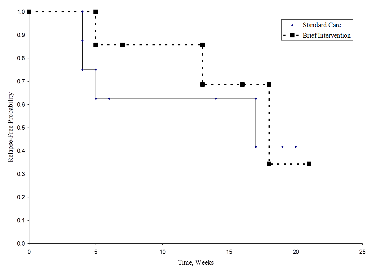
The figure below shows the survival (relapse-free time) in each group. Notice that the survival curves do not show much separation, consistent with the non-significant findings in the test of hypothesis.
Relapse-Free Time in Each Group
As noted, there are several variations of the log rank statistic. Some statistical computing packages use the following test statistic for the log rank test to compare two independent groups:
where ΣO1t is the sum of the observed number of events in group 1, and ΣE1t is the sum of the expected number of events in group 1 taken over all event times. The denominator is the sum of the variances of the expected numbers of events at each event time, which is computed as follows:
There are other versions of the log rank statistic as well as other tests to compare survival functions between independent groups.7-9 For example, a popular test is the modified Wilcoxon test which is sensitive to larger differences in hazards earlier as opposed to later in follow-up.10