Screening for Disease
Without screening, diagnosis of disease only occurs after symptoms develop. However, disease frequently begins long before symptoms occur, and even in the absence of symptoms there may be a point at which the disease could be detected by a screening test. The time interval between possible detection by screening and later detection after symptoms is the "detectable pre-clinical phase" or DPCP. We hope that detection of disease in the DPCP will lead to earlier treatment and that this, in turn, will lead to a better outcome. However, this is not always the case. There has been much controversy regarding the age at which routine mammography screening should begin in order to screen for breast cancer. More recently, there has been controversy about whether PSA (prostate-specific antigen) screening should be used at all in men.
After completing this module, the student will be able to:

Without screening, diagnosis of disease only occurs after symptoms develop. However, disease frequently begins long before symptoms occur, and even in the absence of symptoms there may be a point at which the disease could be detected by a screening test. The time interval between possible detection by screening and later detection after symptoms is the "detectable pre-clinical phase" or DPCP. We hope that detection of disease in the DPCP will lead to earlier treatment and that this, in turn, will lead to a better outcome. However, this is not always the case.
By these criteria, blood pressure screening to detect and treat hypertension is an ideal circumstance for screening.
However,screening is not always appropriate:
If a test is reliable, it gives consistent results with repeated tests. Variability in the measurement can be the result of physiologic variation or the result of variables related to the method of testing. For example, if one were using a sphygmomanometer to measure blood pressure repeatedly over time in a single individual, the results might vary depending on:
The reliability of all tests can potential be affected by one or more of these factors.
Test validity is the ability of a screening test to accurately identify diseased and non-disease individuals. An ideal screening test is exquisitely sensitive (high probability of detecting disease) and extremely specific (high probability that those without the disease will screen negative). However, there is rarely a clean distinction between "normal" and "abnormal."
The validity of a screening test is based on its accuracy in identifying diseased and non-diseased persons, and this can only be determined if the accuracy of the screening test can be compared to some "gold standard" that establishes the true disease status. The gold standard might be a very accurate, but more expensive diagnostic test. Alternatively, it might be the final diagnosis based on a series of diagnostic tests. If there were no definitive tests that were feasible or if the gold standard diagnosis was invasive, such as a surgical excision, the true disease status might only be determined by following the subjects for a period of time to determine which patients ultimately developed the disease. For example, the accuracy of mammography for breast cancer would have to be determined by following the subjects for several years to see whether a cancer was actually present.
A 2 x 2 table, or contingency table, is also used when testing the validity of a screening test, but note that this is a different contingency table than the ones used for summarizing cohort studies, randomized clinical trials, and case-control studies. The 2 x 2 table below shows the results of the evaluation of a screening test for breast cancer among 64,810 subjects.
|
|
Diseased |
Not Diseased |
Total |
|---|---|---|---|
|
Test Positive |
132 |
983 |
1,115 |
|
Test Negative |
45 |
63,650 |
63,695 |
|
Column Totals |
177 |
64,633 |
64,810 |
The contingency table for evaluating a screening test lists the true disease status in the columns, and the observed screening test results are listed in the rows. The table shown above shows the results for a screening test for breast cancer. There were 177 women who were ultimately found to have had breast cancer, and 64,633 women remained free of breast cancer during the study. Among the 177 women with breast cancer, 132 had a positive screening test (true positives), but 45 had negative tests (false negatives). Among the 64,633 women without breast cancer, 63,650 appropriately had negative screening tests (true negatives), but 983 incorrectly had positive screening tests (false positives).
If we focus on the rows, we find that 1,115 subjects had a positive screening disease, i.e., the test results were abnormal and suggested disease. However, only 132 of these were found to actually have disease, based on the gold standard test. Also note that 63,695 people had a negative screening test, suggesting that they did not have the disease, BUT, in fact 45 of these people were actually diseased.
One measure of test validity is sensitivity, i.e., how accurate the screening test is in identifying disease in people who truly have the disease. When thinking about sensitivity, focus on the individuals who, in fact, really were diseased - in this case, the left hand column.
Table - Illustration of the Sensitivity of a Screening Test
|
|
Diseased |
Not Diseased |
Total |
|---|---|---|---|
|
Test Positive |
132 |
983 |
1,115 |
|
Test Negative |
45 |
63,650 |
63,695 |
|
Column Totals |
177 |
64,633 |
64,810 |
What was the probability that the screening test would correctly indicate disease in this subset? The probability is simply the percentage of diseased people who had a positive screening test, i.e., 132/177 = 74.6%. I could interpret this by saying, "The probability of the screening test correctly identifying diseased subjects was 74.6%."
Specificity focuses on the accuracy of the screening test in correctly classifying truly non-diseased people. It is the probability that non-diseased subjects will be classified as normal by the screening test.
Table - Illustration of the Specificity of a Screening Test
|
|
Diseased |
Not Diseased |
Total |
|---|---|---|---|
|
Test Positive |
132 |
983 |
1,115 |
|
Test Negative |
45 |
63,650 |
63,695 |
|
Column Totals |
177 |
64,633 |
64,810 |
As noted in the biostatistics module on Probability,
Link to the biostatistics module on Probability,
In this example, the specificity is 63,650/64,633 = 98.5%. I could interpret this by saying, "The probability of the screening test correctly identifying non-diseased subjects was 98.5%."

Question: In the above example, what was the prevalence of disease among the 64,810 people in the study population? Compute the answer on your own before looking at the answer.
Answer
(Or the Criterion of "Normal")
One problem is that a decision must be made about what test value will be used to distinguish normal versus abnormal results. Unfortunately, when we compare the distributions of screening measurements in subjects with and without disease, we find that there is almost always some overlap, as shown in the figure to the right. Deciding the criterion for "normal" versus abnormal can be difficult.
Figure 16-5 in the textbook by Aschengrau and Seage summarizes the problem.
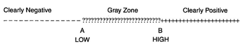
There may be a very low range of test results (e.g., below point A in the figure above) that indicates absence of disease with very high probability, and there may be a very high range (e.g., above point B) that indicates the presence of disease with very high probability. However, where the distributions overlap, there is a "gray zone" in which there is much less certainly about the results.
Consider the example illustrated by the next figure.
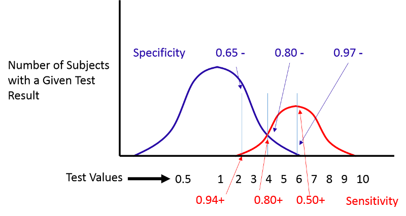
If we move the cut-off to the left, we can increase the sensitivity, but the specificity will be worse. If we move the cut-off to the right, the specificity will improve, but the sensitivity will be worse. Altering the criterion for a positive test ("abnormality") will always influence both the sensitivity and specificity of the test.
(Receiver Operating Characteristic Curves)
(NOTE: You will not be tested on ROC curves in the introductory course.)
ROC curves provide a means of defining the criterion of positivity that maximizes test accuracy when the test values in diseased and non-diseased subjects overlap. As the previous figure demonstrates, one could select several different criteria of positivity and compute the sensitivity and specificity that would result from each cut point. In the example above, suppose I computed the sensitivity and specificity that would result if I used cut points of 2, 4, or 6. If I were to do this for the example above, by table would look something like this:
|
Criterion of Positivity |
Sensitivity (True Positive Rate) |
Specificity |
False Positive Rate (1-Specificity) |
|---|---|---|---|
|
2 |
0.94 |
0.65 |
0.35 |
|
4 |
0.80 |
0.80 |
0.20 |
|
6 |
0.50 |
0.97 |
0.03 |
I could then plot the true positive rate (the sensitivity) as a function of the false positive rate (1-specificity), and the plot would look like the figure below.
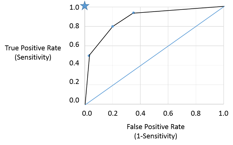
Note that the true positive and false positive rates obtained with the three different cut points (criteria) are are shown by the three blue points representing true positive and false positive rates using the three different criteria of positivity. This is a receiver-operator characteristic curve that assesses test accuracy by looking at how true positive and false positive rates change when different criteria of positivity are used. If the diseased people had test values that were always greater than the test values in non-diseased people, i.e., there were two entirely separate distributions then one could easily select a criterion of positivity that gave a true positive rate of 1 (100%) and a false positive rate of 0, as depicted by the blue star at the upper left hand corner (coordinates 0,1). The closer the ROC curve hugs the left axis and the top border, the more accurate the test, i.e., the closer the curve is to the star. The diagonal blue line illustrates the ROC curve for a useless test for which the true positive rate and the false positive rate are equal regardless of the criterion of positivity that is used - in other words the distribution of test values for disease and non-diseased people overlap entirely. So, the closer the ROC curve is to the blue star, the better it is, and the closer it is to the diagonally blue line, the worse it is.
This provides a standard way of assessing test accuracy, but perhaps another approach might be to consider the seriousness of the consequences of a false negative test. For example, failing to identify diabetes right away from a dip stick test of urine would not necessarily have any serious consequences in the long run, but failing to identify a condition that was more rapidly fatal or had serious disabling consequences would be much worse. Consequently, a common sense approach might be to select a criterion that maximizes sensitivity and accept the if the higher false positive rate that goes with that if the condition is very serious and would benefit the patient if diagnosed early.
Here is a link to a journal article describing a study looking at sensitivity and specificity of PSA testing for prostate cancer. [Richard M Hoffman, Frank D Gilliland, et al.: Prostate-specific antigen testing accuracy in community practice. BMC Family Practice 2002, 3:19]
In the video below Dr. David Felson from the Boston University School of Medicine discusses sensitivity and specificity of screening tests and diagnostic tests.
When evaluating the feasibility or the success of a screening program, one should also consider the positive and negative predictive values. These are also computed from the same 2 x 2 contingency table, but the perspective is entirely different.
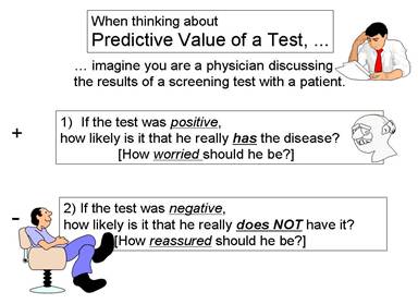
One way to avoid confusing this with sensitivity and specificity is to imagine that you are a patient and you have just received the results of your screening test (or imagine you are the physician telling a patient about their screening test results. If the test was positive, the patient will want to know the probability that they really have the disease, i.e., how worried should they be?
Conversely, if it is good news, and the screening test was negative, how reassured should the patient be? What is the probability that they are disease free?
Another way that helps me keep this straight is to always orient my contingency table with the gold standard at the top and the true disease status listed in the columns. The illustrations used earlier for sensitivity and specificity emphasized a focus on the numbers in the left column for sensitivity and the right column for specificity. If this orientation is used consistently, the focus for predictive value is on what is going on within each row in the 2 x 2 table, as you will see below.
If a test subject has an abnormal screening test (i.e., it's positive), what is the probability that the subject really has the disease? In the example we have been using there were 1,115 subjects whose screening test was positive, but only 132 of these actually had the disease, according to the gold standard diagnosis. Therefore, if a subject's screening test was positive, the probability of disease was 132/1,115 = 11.8%.
Table - Illustration of Positive Predicative Value of a Hypothetical Screening Test
|
|
Diseased |
Not Diseased |
Total |
|---|---|---|---|
|
Test Positive |
132 |
983 |
1,115 |
|
Test Negative |
45 |
63,650 |
63,695 |
|
Column Totals |
177 |
64,633 |
64,810 |
Here, the positive predictive value is 132/1,115 = 0.118, or 11.8%.
Interpretation: Among those who had a positive screening test, the probability of disease was 11.8%.
Negative predictive value: If a test subject has a negative screening test, what is the probability that the subject really does not have the disease? In the same example, there were 63,895 subjects whose screening test was negative, and 63,650 of these were, in fact, free of disease. Consequently, the negative predictive value of the test was 63,650/63,695 = 99.9%.
Table - Illustration of Negative Predicative Value of a Hypothetical Screening Test
|
|
Diseased |
Not Diseased |
Total |
|---|---|---|---|
|
Test Positive |
132 |
983 |
1,115 |
|
Test Negative |
45 |
63,650 |
63,695 |
|
Column Totals |
177 |
64,633 |
64,810 |
Here, the négative predictive values is 63,650/63,950=0.999, or 99.9%.
Interpretation: Among those who had a negative screening test, the probability of being disease-free was 99.9%.
This widget will compute sensitivity, specificity, and positive and negative predictive value for you. Just enter the results of a screening evaluation into the turquoise cells.
Optional
Dr. David Felson is a Professor of Medicine in the Boston University School of Medicine, and he teaches a course in Clinical Epidemiology at the BU School of Public Health. In the video below, he discusses predictive value.
One factor that influences the feasibility of a screening program is the yield, i.e., the number of cases detected. This can be estimated from the positive predictive value.
Sensitivity and specificity are characteristics of the test and are only influenced by the test characteristics and the criterion of positivity that is selected. In contrast, the positive predictive value of a test, or the yield, is very dependent on the prevalence of the disease in the population being tested. The higher the prevalence of disease is in the population being screened, the higher the positive predictive values (and the yield). Consequently, the primary means of increasing the yield of a screening program is to target the test to groups of people who are at higher risk of developing the disease.
To illustrate the effect of prevalence on positive predictive value, consider the yield that would be obtained for HIV testing in three different settings. Serological testing for HIV is extremely sensitive (100%) and specific (99.5%), but the positive predictive value of HIV testing will vary markedly depending on the prevalence of pre-clinical disease in the population being tested. The examples below show how drastically the predicative value varies among three groups of test subjects.
These three scenarios all illustrate the consequences of HIV testing using a test that is 100% sensitive and 99.5% specific. All three show the effects of screening 100,000 subjects. The only thing that is different among these three populations is the prevalence of previously undiagnosed HIV.
Screening Program #1
The 1st scenario illustrates the yield if the screening program were conducted in female blood donors, in whom the prevalence of disease is only 0.01%. Even with 100% sensitivity and 95% specificity, the positive predictive value (yield) is only 1.9%.
Table - HIV Screening in a Population With HIV Prevalence of Female Blood Donors
|
|
Really HIV+ |
Really HIV- |
Row Totals |
|---|---|---|---|
|
Screen Test + |
10 |
510 |
520 |
|
Screen Test - |
0 |
99,480 |
99,480 |
|
Column Totals |
10 |
99,990 |
100,000 |
Prevalence is 10/100,000 = 0.01%
Positive predictive value = 10/520=0.019, or 1.9%
Screening Program #2
The 2nd scenario illustrates the yield if the screening program were conducted in males in a clinic for sexually transmitted infections, in whom the prevalence of disease is 4%. With the same sensitivity and specificity, the positive predictive value (yield) is 89%.
Table - HIV Screening in a Population of Males Visiting Clinics for Sexual Transmitted Diseases
|
|
Really HIV+ |
Really HIV- |
Row Totals |
|---|---|---|---|
|
Screen Test + |
4,000 |
480 |
4,480 |
|
Screen Test - |
0 |
95,520 |
95,520 |
|
Column Totals |
4,000 |
96,000 |
100,000 |
Prevalence in males visiting clinics for sexual transmitted disease = 4,000/100,000=0.04, or 4%
Positive predictive value = 4000/4480 = 0.83, or 83%
Screening Program #3
Table - HIV Screening in a Population of Intravenous Drug Users
|
|
Really HIV+ |
Really HIV- |
Row Totals |
|---|---|---|---|
|
Screen Test + |
20,000 |
400 |
20,400 |
|
Screen Test - |
0 |
79,600 |
79,600 |
|
|
20,000 |
80,000 |
100,000 |
Prevalence of HIV in these IV Drug Users = 20,000/100,000 = 0.20, or 20%
Positive predictive value = 20,000/20,400 = 0.98, or 98%
This 3rd scenario illustrates the yield if the screening program were conducted in users of intravenous drugs, in whom the prevalence of disease is 20%. With the same sensitivity and specificity, the positive predictive value (yield) is 98%.
What these three scenarios illustrate is that if you have limited resources for screening, and you want to get the most "bang for the buck," target a subset of the population that is likely to have a higher prevalence of disease, and don't screen subsets who are very unlikely to be diseased.
[From Richard M Hoffman, Frank D Gilliland, et al.: Prostate-specific antigen testing accuracy in community practice. BMC Family Practice 2002, 3:19]
"Methods: PSA testing results were compared with a reference standard of prostate biopsy. Subjects were 2,620 men 40 years and older undergoing (PSA) testing and biopsy from 1/1/95 through 12/31/98 in the Albuquerque, New Mexico metropolitan area. Diagnostic measures included the area under the receiver-operating characteristic curve, sensitivity, specificity, and likelihood ratios.
Results: Cancer was detected in 930 subjects (35%). The area under the ROC curve was 0.67 and the PSA cut point of 4 ng/ml had a sensitivity of 86% and a specificity of 33%."
Question: What was the positive predictive value in this study? Hint: You have to use the information provided to piece together the complete 2x2 table; then compute the PPV. See if you can do this before looking at the answer.
Answer
Optional
Dr. David Felson is a Professor of Medicine in the Boston University School of Medicine, and he teaches a course in Clinical Epidemiology at the BU School of Public Health. In the video below, he discusses serial and parallel diagnostic testing.
At first glance screening would seem to be a good thing to do, but there are consequences to screening that carry a cost, and the potential benefits of screening need to be weighed against the risks, especially in subsets of the population that have low prevalence of disease!
There are two important down sides to screening:
Specifically, one needs to consider what happens to the people who had a positive screening test but turned out not to have the disease (false positives). Women between 20-30 years old can get breast cancer, but the probability is extremely low (and the sensitivity of mammography is low because younger women have denser breast tissue). Not only will the yield be low, but many of the false positives will be subjected to extreme anxiety and worry. They may also undergo invasive diagnostic tests such as needle biopsy and surgical biopsy unnecessarily. In the case of fecal blood testing for colorectal cancer, patients with positive screening tests will undergo colonoscopy, which is expensive, inconvenient, and uncomfortable, and it carries its own risks such as accidental perforation of the colon. Such complications are uncommon, but they do occur. The other problem is false negatives, who will be reassured that they don't have disease, when they really do. These hazards of screening must be considered before a screening program is undertaken.
For a very relevant look at this, see the following brief article from the New York Times on the potential harms of screening for prostate cancer. Link to the article
There is concern among some that there is an inordinate emphasis on early diagnosis of disease and that the increasingly aggressive pursuit of abnormalities among people without symptoms is leading to actually harm and great cost without reaping any benefits. For an interesting perspective, see the following essay, Link to "What's Making Us Sick Is an Epidemic of Diagnoses," in the New York Times by Gilbert Welch, Lisa Schwartz, and Steven Woloshin.
This is an article in the New York Times (Tara Parker-Pope: Link to "Scientists Seek to Rein In Diagnoses of Cancer") in which the problem of over-diagnosis is discussed.
Even if a test accurately and efficiently identifies people with pre-clinical disease, its effectiveness is ultimately measured by its ability to reduce morbidity and mortality of the disease. The most definitive measure of efficacy is the difference in cause-specific mortality between those diagnosed by screening versus those diagnosed by symptoms. There are several study designs which can potentially be used to evaluate the efficacy of screening.
These include correlational studies that examine trends in disease-specific mortality over time, correlating them with the frequency of screening in a population. However,1) these are measures for entire populations, and cannot establish that decreased mortality is occurring among those being screened; 2) one cannot adjust for confounding; and 3) one cannot determine optimal screening strategies for subsets of the population.
Case-control and cohort studies are frequently used to evaluate screening, but their chief limitation is that the study groups may not be comparable because of confounders, volunteer bias, lead-time bias, and length-time bias.
Because of these limitations, the optimal means of evaluating efficacy of a screening program is to conduct a randomized clinical trial (RCT) with a large enough sample to ensure control of potential confounding factors. However, the costs and ethical problems associated with RCTs for screening can be substantial, and much data will continue to come from observational studies. Screening programs also tend to look better than they really are because of several factors:
People who choose to participate in screening programs tend to be healthier, have healthier lifestyles, and they tend to adhere to therapy better, and their outcomes tend to be better because of this. However, volunteers may also represent the "worried well," i.e., people who are asymptomatic, but at higher risk (e.g., relatives of women with breast cancer). All of these factors can bias the apparent benefit of screening.
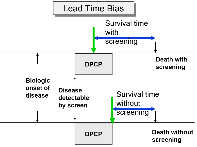
The premise of screening is that it allows you to identify disease earlier, so you can initiate treatment at an early stage in order to effect cure or at least longer survival. Screening can give you a jump on the disease; this "lead-time" is a good thing, but it can bias the efficacy of screening. The two subjects to the right have the same age, same time of disease onset, the same DPCP, and the same time of death. However, if we compare survival time from the point of diagnosis, the subject whose disease was identified through screening appears to survive longer, but only because their disease was identified earlier.
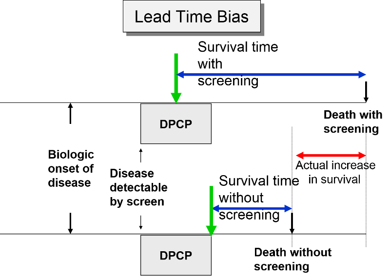
In the next figure two patients again have identical biologic onset and detectable pre-clinical phases. In this case the screened patient lives longer than the unscreened patient, but his survival time is still exaggerated by the lead time from earlier diagnosis.
The length of the DPCP can vary substantially from person to person. Prostate cancer, for example, is a very slow growing tumor in many men, but very rapidly progressing and lethal in others. These differences in DPCP exaggerate the apparent benefit of screening, because there is a greater chance that screening will detect subjects with long DPCPs, and therefore, more benign disease.
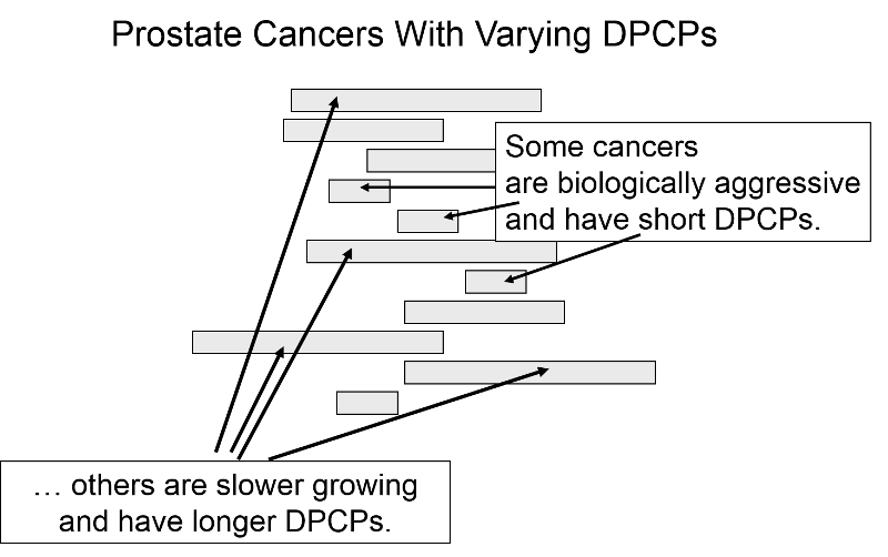
To illustrate consider a hypothetical randomized trial in which half of the subjects were screened and the other half were not. Because we assigned subjects randomly, the DPCPs are more or less equally distributed in the two groups. If we conduct a screening in half of the subjects at a specific point in time, there is a greater probability that those who screen positive will have longer DPCPs on average, because they are detectable by screening, but their disease has not progressed to the stage of causing symptoms or death yet.
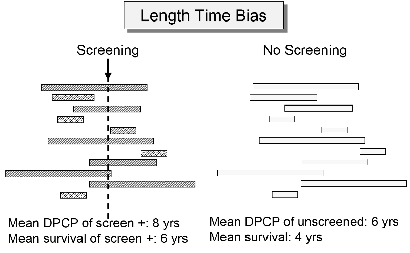
The unscreened population will include an assortment of subjects with long and short DPCPs, and they will all be identified by their symptoms and/or death. The screened subjects who are identified as having disease will tend to have longer survival times, because they have, on average, a less aggressive form of cancer.
For an nice summary of lead time bias, and length time bias follow this link: Primer on Lead-Time, Length, and Overdiagnosis Bias.
Down syndrome is a spectrum of abnormalities that generally result from an error during gametogenesis in the ovary that results in the birth of a child with three copies of chromosome 21 (trisomy 21) instead of the normal two copies. The frame below from the National Institutes of Health provides a summary of the syndrome.
Prior to 2014 the most up-to-date screening method during pregnancy was a combined approach during the first trimester that was conducted in two steps during week 11 to 13 during pregnancy.
In late 2011 cell-free DNA sequencing (cfDNA testing) of maternal plasma was introduced as a new screening modality in the US. Bianchi et al. reported on results with the new screening test among 2052 women with singleton pregnancies who were enrolled in the study.
This link below will allow you to listen to a report about the study on National Public Radio (NPR).
The tables below summarize the evaluations of the "Standard Test for Down syndrome and the results obtained with the newer DNA sequencing technique.
Standard Test
|
|
Down Syndrome |
Not Down |
|
Test + |
5 |
69 |
|
Test - |
0 |
1835 |
|
|
5 |
1904 |
DNA Sequencing
|
|
Down Syndrome |
Not Down |
|
Test + |
5 |
6 |
|
Test - |
0 |
1898 |
|
|
5 |
1904 |
At first glance, the results look pretty similar. Compute the sensitivity, specificity, and positive predictive value of each screening test and comment on the utility of the newer DNA test compared to the previous standard testing.
Answer
Articles addressing some of the controversies in screening for disease:
Mammography Screening for Breast Cancer
Cervical Cancer
PSA Screening for Prostate Cancer
Subjects were 2,620 men 40 years and older undergoing (PSA) testing and biopsy.
Cancer was detected in 930 subjects (35%). The area under the ROC curve was 0.67 and the PSA cut point of 4 ng/ml had a sensitivity of 86% and a specificity of 33%. What was the positive predictive value in this study?
Answer:
The area under the ROC curve is irrelevant. The question gives us the total number of subjects and the prevalence of biopsy-proven prostate cancer. It also gives us the sensitivity and specificity of the the PSA test that they used, so we can construct the contingency table from this information, and then compute the positive predictive value.
There were 930 men with confirmed prostate cancer, so this is the column total for cancer. If the sensitivity was 86%, then the number of diseased men with a positive test was 0.86 x 930 = 799.8 or 800 men. Therefore, the other 130 men with prostate cancer must have had a negative PSA test. If the study consisted of 2,620 men and 930 had cancer, then there must have been 2,620-930= 1690 men without cancer. And if the specificity was 33%, then there must have been 0.33 x 1690= 557.8 or 558 men without cancer who had negative PSA tests. Therefore, the number of men without prostate cancer who had positive tests must have been 1690-558=1132.
From this information we can now construct our screening contingency table as shown below. The last column was computed by adding the numbers in columns 2 and 3.
Table - Results of Screening for Prostate Cancer with Prostate-specific Antigen Test
|
|
Biopsy-proven Cancer |
No Cancer |
Row Totals |
|---|---|---|---|
|
PSA Screen + |
800 |
1,132 |
1,932 |
|
PSA Screen - |
130 |
558 |
688 |
|
Column Totals |
930 |
1,690 |
2,620 |
Given these data, the positive predictive value is 800/1932 = 0.42, or 42%.
Interpretation: The probability of biopsy-proven prostate cancer among men with a positive PSA test was 42%.
The negative predictive value was 558/688 = 0.81, or 81%.
Interpretation: The probability of not having prostate cancer among men with a negative PSA test was 81%.
Sensitivity = 5/5 = 100%
Specificity = 1835/1904 = 96.4%
Positive Predictive Value = 5/74 = 6.8%
DNA Sequencing
Sensitivity = 5/5 = 100% Specificity = 1898/1904= 99.7% Positive Predictive Value = 5/11 = 45.5%
Both tests had a sensitivity of 100%. However, as suggested by the NPR broadcast, the specificity of the new test that used DNA sequencing was better and resulted on only 6 false positive screening tests compared to 69 false positive tests with the older standard test. Since women with positive screening tests are recommended to undergo amniocentesis for definitive diagnosis, false positive tests in this setting represent cases in which unnecessary amniocentesis was done, placing the fetus at risk.
Note that amniocentesis is expensive and anxiety-producing, and it can cause a miscarriage (risk of 0.25-0.5%). Other rare complications of amniocentesis include Injury to the baby or mother, infection, and pre-term labor.