Case-Control Studies
Cohort studies have an intuitive logic to them, but they can be very problematic when one is investigating outcomes that only occur in a small fraction of exposed and unexposed individuals. They can also be problematic when it is expensive or very difficult to obtain exposure information from a cohort. In these situations a case-control design offers an alternative that is much more efficient. The goal of a case-control study is the same as that of cohort studies, i.e., to estimate the magnitude of association between an exposure and an outcome. However, case-control studies employ a different sampling strategy that gives them greater efficiency.
After completing this module, the student will be able to:

In the module entitled Overview of Analytic Studies it was noted that Rothman describes the case-control strategy as follows:
"Case-control studies are best understood by considering as the starting point a source population, which represents a hypothetical study population in which a cohort study might have been conducted. The source population is the population that gives rise to the cases included in the study. If a cohort study were undertaken, we would define the exposed and unexposed cohorts (or several cohorts) and from these populations obtain denominators for the incidence rates or risks that would be calculated for each cohort. We would then identify the number of cases occurring in each cohort and calculate the risk or incidence rate for each. In a case-control study the same cases are identified and classified as to whether they belong to the exposed or unexposed cohort. Instead of obtaining the denominators for the rates or risks, however, a control group is sampled from the entire source population that gives rise to the cases. Individuals in the control group are then classified into exposed and unexposed categories. The purpose of the control group is to determine the relative size of the exposed and unexposed components of the source population. Because the control group is used to estimate the distribution of exposure in the source population, the cardinal requirement of control selection is that the controls be sampled independently of exposure status."
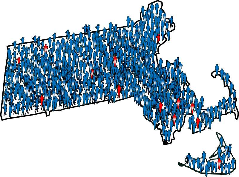
To illustrate this consider the following hypothetical scenario in which the source population is the state of Massachusetts. Diseased individuals are red, and non-diseased individuals are blue. Exposed individuals are indicated by a whitish midsection. Note the following aspects of the depicted scenario:
If we somehow had exposure and outcome information on all of the subjects in the source population and looked at the association using a cohort design, we might find the data summarized in the contingency table below.
|
|
Diseased |
Non-diseased |
Total |
|---|---|---|---|
|
Exposed |
700 |
999,300 |
1,000,000 |
|
Non-exposed |
600 |
4,999,400 |
5,000,000 |
In this hypothetical example, we have data on all 6,000,000 people in the source population, and we could compute the probability of disease (i.e., the risk or incidence) in both the exposed group and the non-exposed group, because we have the denominators for both the exposed and non-exposed groups.
The table above summarizes all of the necessary information regarding exposure and outcome status for the population and enables us to compute a risk ratio as a measure of the strength of the association. Intuitively, we compute the probability of disease (the risk) in each exposure group and then compute the risk ratio as follows:
The problem, of course, is that we usually don't have the resources to get the data on all subjects in the population. If we took a random sample of even 5-10% of the population, we would have few diseased people in our sample, certainly not enough to produce a reasonably precise measure of association. Moreover, we would expend an inordinate amount of effort and money collecting exposure and outcome data on a large number of people who would not develop the outcome.
We need a method that allows us to retain all the people in the numerator of disease frequency (diseased people or "cases") but allows us to collect information from only a small proportion of the people that make up the denominator (population, or "controls"), most of whom do not have the disease of interest. The case-control design allows us to accomplish this. We identify and collect exposure information on all the cases, but identify and collect exposure information on only a sample of the population. Once we have the exposure information, we can assign subjects to the numerator and denominator of the exposed and unexposed groups. This is what Rothman means when he says,
"The purpose of the control group is to determine the relative size of the exposed and unexposed components of the source population."
In the above example, we would have identified all 1,300 cases, determined their exposure status, and ended up categorizing 700 as exposed and 600 as unexposed. We might have ransomly sampled 6,000 members of the population (instead of 6 million) in order to determine the exposure distribution in the total population. If our sampling method was random, we would expect that about 1,000 would be exposed and 5,000 unexposed (the same ratio as in the overall population). We calculate a similar measure as the risk ratio above, but substituting in the denominator a sample of the population ("controls") instead of the whole population:
Note that when we take a sample of the population, we no longer have a measure of disease frequency, because the denominator no longer represents the population. Therefore, we can no longer compute the probability or rate of disease incidence in each exposure group. We also can't calculate a risk or rate difference measure for the same reason. However, as we have seen, we can compute the relative probability of disease in the exposed vs. unexposed group. The term generally used for this measure is an odds ratio, described in more detail later in the module.
Consequently, when the outcome is uncommon, as in this case, the risk ratio can be estimated much more efficiently by using a case-control design. One would focus first on finding an adequate number of cases in order to determine the ratio of exposed to unexposed cases. Then, one only needs to take a sample of the population in order to estimate the relative size of the exposed and unexposed components of the source population. Note that if one can identify all of the cases that were reported to a registry or other database within a defined period of time, then it is possible to compute an estimate of the incidence of disease if the size of the population is known from census data. While this is conceptually possible, it is rarely done, and we will not discuss it further in this course.


Suppose a prospective cohort study were conducted among almost 90,000 women for the purpose of studying the determinants of cancer and cardiovascular disease. After enrollment, the women provide baseline information on a host of exposures, and they also provide baseline blood and urine samples that are frozen for possible future use. The women are then followed, and, after about eight years, the investigators want to test the hypothesis that past exposure to pesticides such as DDT is a risk factor for breast cancer. Eight years have passed since the beginning of the study, and 1.439 women in the cohort have developed breast cancer. Since they froze blood samples at baseline, they have the option of analyzing all of the blood samples in order to ascertain exposure to DDT at the beginning of the study before any cancers occurred. The problem is that there are almost 90,000 women and it would cost $20 to analyze each of the blood samples. If the investigators could have analyzed all 90,000 samples this is what they would have found the results in the table below.
Table of Breast Cancer Occurrence Among Women With or Without DDT Exposure
|
|
Breast Cancer |
No Breast Cancer |
Total |
|---|---|---|---|
|
DDT exposed |
360 |
13,276 |
13,636 |
|
Unexposed |
1,079 |
75,234 |
76,313 |
|
|
1,439 |
88,510 |
89,949 |
Hypothetical: 
If they had been able to afford analyzing all of the baseline blood specimens in order to categorize the women as having had DDT exposure or not, they would have found a risk ratio = 1.87 (95% confidence interval: 1.66-2.10). The problem is that this would have cost almost $1.8 million, and the investigators did not have the funding to do this.
While 1,439 breast cancers is a disturbing number, it is only 1.6% of the entire cohort, so the outcome is relatively rare, and it is costing a lot of money to analyze the blood specimens obtained from all of the non-diseased women. There is, however, another more efficient alternative, i.e., to use a case-control sampling strategy. One could analyze all of the blood samples from women who had developed breast cancer, but only a sample of the whole cohort in order to estimate the exposure distribution in the population that produced the cases.
If one were to analyze the blood samples of 2,878 of the non-diseased women (twice as many as the number of cases), one would obtain results that would look something like those in the next table.
Table of Breast Cancer Occurrence Among Women With or Without DDT Exposure
|
|
Breast Cancer |
No Breast Cancer |
|---|---|---|
|
DDT exposed |
360 |
432 |
|
Unexposed |
1,079 |
2,446 |
|
|
1,439 |
2,878 |
Odds of Exposure: 360/1079 in the cases versus 432/2,446 in the non-diseased controls.
Totals Samples analyzed = 1,438+2,878 = 4,316
Total Cost = 4,316 x $20 = $86,320
With this approach a similar estimate of risk was obtained after analyzing blood samples from only a small sample of the entire population at a fraction of the cost with hardly any loss in precision. In essence, a case-control strategy was used, but it was conducted within the context of a prospective cohort study. This is referred to as a case-control study "nested" within a cohort study.
Rothman states that one should look upon all case-control studies as being "nested" within a cohort. In other words the cohort represents the source population that gave rise to the cases. With a case-control sampling strategy one simply takes a sample of the population in order to obtain an estimate of the exposure distribution within the population that gave rise to the cases. Obviously, this is a much more efficient design.
It is important to note that, unlike cohort studies, case-control studies do not follow subjects through time. Cases are enrolled at the time they develop disease and controls are enrolled at the same time. The exposure status of each is determined, but they are not followed into the future for further development of disease.
As with cohort studies, case-control studies can be prospective or retrospective. At the start of the study, all cases might have already occurred and then this would be a retrospective case-control study. Alternatively, none of the cases might have already occurred, and new cases will be enrolled prospectively. Epidemiologists generally prefer the prospective approach because it has fewer biases, but it is more expensive and sometimes not possible. When conducted prospectively, or when nested in a prospective cohort study, it is straightforward to select controls from the population at risk. However, in retrospective case-control studies, it can be difficult to select from the population at risk, and controls are then selected from those in the population who didn't develop disease. Using only the non-diseased to select controls as opposed to the whole population means the denominator is not really a measure of disease frequency, but when the disease is rare, the odds ratio using the non-diseased will be very similar to the estimate obtained when the entire population is used to sample for controls. This phenomenon is known as the rare-disease assumption. When case-control studies were first developed, most were conducted retrospectively, and it is sometimes assumed that the rare-disease assumption applies to all case-control studies. However, it actually only applies to those case-control studies in which controls are sampled only from the non-diseased rather than the whole population.
The difference between sampling from the whole population and only the non-diseased is that the whole population contains people both with and without the disease of interest. This means that a sampling strategy that uses the whole population as its source must allow for the fact that people who develop the disease of interest can be selected as controls. Students often have a difficult time with this concept. It is helpful to remember that it seems natural that the population denominator includes people who develop the disease in a cohort study. If a case-control study is a more efficient way to obtain the information from a cohort study, then perhaps it is not so strange that the denominator in a case-control study also can include people who develop the disease. This topic is covered in more detail in EP813 Intermediate Epidemiology.
Students usually think of case-control studies as being only retrospective, since the investigators enroll subjects who have developed the outcome of interest. However, case-control studies, like cohort studies, can be either retrospective or prospective. In a prospective case-control study, the investigator still enrolls based on outcome status, but the investigator must wait to the cases to occur.
Given the greater efficiency of case-control studies, they are particularly advantageous in the following situations:
Another advantage of their greater efficiency, of course, is that they are less time-consuming and much less costly than prospective cohort studies.
A classic example of the efficiency of the case-control approach is the study (Herbst et al.: N. Engl. J. Med. Herbst et al. (1971;284:878-81) that linked in-utero exposure to diethylstilbesterol (DES) with subsequent development of vaginal cancer 15-22 years later. In the late 1960s, physicians at MGH identified a very unusual cancer cluster. Eight young woman between the ages of 15-22 were found to have cancer of the vagina, an uncommon cancer even in elderly women. The cluster of cases in young women was initially reported as a case series, but there were no strong hypotheses about the cause.
In retrospect, the cause was in-utero exposure to DES. After World War II, DES started being prescribed for women who were having troubles with a pregnancy -- if there were signs suggesting the possibility of a miscarriage, DES was frequently prescribed. It has been estimated that between 1945-1950 DES was prescribed for about 20% of all pregnancies in the Boston area. Thus, the unborn fetus was exposed to DES in utero, and in a very small percentage of cases this resulted in development of vaginal cancer when the child was 15-22 years old (a very long latent period). There were several reasons why a case-control study was the only feasible way to identify this association: the disease was extremely rare (even in subjects who had been exposed to DES), there was a very long latent period between exposure and development of disease, and initially they had no idea what was responsible, so there were many possible exposures to consider.
In this situation, a case-control study was the only reasonable approach to identify the causative agent. Given how uncommon the outcome was, even a large prospective study would have been unlikely to have more than one or two cases, even after 15-20 years of follow-up. Similarly, a retrospective cohort study might have been successful in enrolling a large number of subjects, but the outcome of interest was so uncommon that few, if any, subjects would have had it. In contrast, a case-control study was conducted in which eight known cases and 32 age-matched controls provided information on many potential exposures. This strategy ultimately allowed the investigators to identify a highly significant association between the mother's treatment with DES during pregnancy and the eventual development of adenocarcinoma of the vagina in their daughters (in-utero at the time of exposure) 15 to 22 years later.
For more information see the DES Fact Sheet from the National Cancer Institute.
An excellent summary of this landmark study and the long-range effects of DES can be found in a Perspective article in the New England Journal of Medicine. A cohort of both mothers who took DES and their children (daughters and sons) was later formed to look for more common outcomes. Members of the faculty at BUSPH are on the team of investigators that follow this cohort for a variety of outcomes, particularly reproductive consequences and other cancers.
Careful thought should be given to the case definition to be used. If the definition is too broad or vague, it is easier to capture people with the outcome of interest, but a loose case definition will also capture people who do not have the disease. On the other hand, an overly restrictive case definition is employed, fewer cases will be captured, and the sample size may be limited. Investigators frequently wrestle with this problem during outbreak investigations. Initially, they will often use a somewhat broad definition in order to identify potential cases. However, as an outbreak investigation progresses, there is a tendency to narrow the case definition to make it more precise and specific, for example by requiring confirmation of the diagnosis by laboratory testing. In general, investigators conducting case-control studies should thoughtfully construct a definition that is as clear and specific as possible without being overly restrictive.
Investigators studying chronic diseases generally prefer newly diagnosed cases, because they tend to be more motivated to participate, may remember relevant exposures more accurately, and because it avoids complicating factors related to selection of longer duration (i.e., prevalent) cases. However, it is sometimes impossible to have an adequate sample size if only recent cases are enrolled.
Typical sources for cases include:
As noted above, it is always useful to think of a case-control study as being nested within some sort of a cohort, i.e., a source population that produced the cases that were identified and enrolled. In view of this there are two key principles that should be followed in selecting controls:
If either of these principles are not adhered to, selection bias can result (as discussed in detail in the module on Bias).
Note that in the earlier example of a case-control study conducted in the Massachusetts population, we specified that our sampling method was random so that exposed and unexposed members of the population had an equal chance of being selected. Therefore, we would expect that about 1,000 would be exposed and 5,000 unexposed (the same ratio as in the whole population), and came up with an odds ratio that was same as the hypothetical risk ratio we would have had if we had collected exposure information from the whole population of six million:
What if we had instead been more likely to sample those who were exposed, so that we instead found 1,500 exposed and 4,500 unexposed among the 6,000 controls? Then the odds ratio would have been:
This odds ratio is biased because it differs from the true odds ratio. In this case, the bias stemmed from the fact that we violated the second principle in selection of controls. Depending on which category is over or under-sampled, this type of bias can result in either an underestimate or an overestimate of the true association.
Example:
A hypothetical case-control study was conducted to determine whether lower socioeconomic status (the exposure) is associated with a higher risk of cervical cancer (the outcome). The "cases" consisted of 250 women with cervical cancer who were referred to Massachusetts General Hospital for treatment for cervical cancer. They were referred from all over the state. The cases were asked a series of questions relating to socioeconomic status (household income, employment, education, etc.). The investigators identified control subjects by going door-to-door in the community around MGH from 9:00 AM to 5:00 PM. Many residents are not home, but they persist and eventually enroll enough controls. The problem is that the controls were selected by a different mechanism than the cases, AND the selection mechanism may have tended to select individuals of different socioeconomic status, since women who were at home may have been somewhat more likely to be unemployed. In other words, the controls were more likely to be enrolled (selected) if they had the exposure of interest (lower socioeconomic status).

A population-based case-control study is one in which the cases come from a precisely defined population, such as a fixed geographic area, and the controls are sampled directly from the same population. In this situation cases might be identified from a state cancer registry, for example, and the comparison group would logically be selected at random from the same source population. Population controls can be identified from voter registration lists, tax rolls, drivers license lists, and telephone directories or by "random digit dialing". Population controls may also be more difficult to obtain, however, because of lack of interest in participating, and there may be recall bias, since population controls are generally healthy and may remember past exposures less accurately.
|
Random Digit Dialing Random digit dialing has been popular in the past, but it is becoming less useful because of the use of caller ID, answer machines, and a greater reliance on cell phones instead of land lines. Ken Rothman points out several that random digit dialing provides an equal probability that any given phone will be dialed, but not an equal probability of reaching eligible control subjects, because households vary in the number of residents and the likelihood that someone will be home. In addition, random digit dialing doesn't make any distinction between residential and business phones.
|
Example of a Population-based Case-Control Study: Rollison et al. reported on a "Population-based Case-Control Study of Diabetes and Breast Cancer Risk in Hispanic and Non-Hispanic White Women Living in US Southwestern States". (ALink to the article - Citation: Am J Epidemiol 2008;167:447–456).
"Briefly, a population-based case-control study of breast cancer was conducted in Colorado, New Mexico, Utah, and selected counties of Arizona. For investigation of differences in the breast cancer risk profiles of non-Hispanic Whites and Hispanics, sampling was stratified by race/ethnicity, and only women who self-reported their race as non-Hispanic White, Hispanic, or American Indian were eligible, with the exception of American Indian women living on reservations. Women diagnosed with histologically confirmed breast cancer between October 1999 and May 2004 (International Classification of Diseases for Oncology codes C50.0–C50.6 and C50.8–C50.9) were identified as cases through population-based cancer registries in each state."
"Population-based controls were frequency-matched to cases in 5-year age groups. In New Mexico and Utah, control participants under age 65 years were randomly selected from driver's license lists; in Arizona and Colorado, controls were randomly selected from commercial mailing lists, since driver's license lists were unavailable. In all states, women aged 65 years or older were randomly selected from the lists of the Centers for Medicare and Medicaid Services (Social Security lists). Of all women contacted, 68 percent of cases and 42 percent of controls participated in the study."
"Odds ratios and 95% confidence intervals were calculated using logistic regression, adjusting for age, body mass index at age 15 years, and parity. Having any type of diabetes was not associated with breast cancer overall (odds ratio = 0.94, 95% confidence interval: 0.78, 1.12). Type 2 diabetes was observed among 19% of Hispanics and 9% of non-Hispanic Whites but was not associated with breast cancer in either group."
In this example, it is clear that the controls were selected from the source population (principle 1), but less clear that they were enrolled independent of exposure status (principle 2), both because drivers' licenses were used for selection and because the participation rate among controls was low. These factors would only matter if they impacted on the estimate of the proportion of the population who had diabetes.
 If cases are obtained from a medical facility, the comparison groups should be obtained from the same facility, provided they meet two criteria:
The advantages of using controls who are patients from the same facility are:
Example: Several years ago the vascular surgeons at Boston Medical Center wanted to study risk factors for severe atherosclerosis of the lower extremities. The cases were patients who were referred to the hospital for elective surgery to bypass severe atherosclerotic blockages in the arteries to the legs. The controls consisted of patients who were admitted to the same hospital for elective joint replacement of the hip or knee. The patients undergoing joint replacement were similar in age and they also were following the same referral pathways. In other words, they met the "would" criterion: if one of the joint replacement surgery patients had developed severe atherosclerosis in their leg arteries, they would have been referred to the same hospital.
Occasionally investigators will ask cases to nominate controls who are in one of these categories, because they have similar characteristics, such as genotype, socioeconomic status, or environment, i.e., factors that can cause confounding, but are hard to measure and adjust for. By matching cases and controls on these factors, confounding by these factors will be controlled. However, one must be careful that the controls satisfy the two fundamental principles. Often, they do not.
Since case-control studies are often used for uncommon outcomes, investigators often have a limited number of cases but a plentiful supply of potential controls. In this situation the statistical power of the study can be increased somewhat by enrolling more controls than cases. However, the additional power that is achieved diminishes as the ratio of controls to cases increases, and ratios greater than 4:1 have little additional impact on power. Consequently, if it is time-consuming or expensive to collect data on controls, the ratio of controls to cases should be no more than 4:1. However, if the data on controls is easily obtained, there is no reason to limit the number of controls.
There are three strategies for selecting controls that are best explained by considering the nested case-control study described on page 3 of this module:
It is often said that an odds ratio provides a good estimate of the risk ratio only when the outcome of interest is rare, but this is only true when survivor sampling is used. With case-base sampling or risk set sampling, the odds ratio will provide a good estimate of the risk ratio regardless of the frequency of the outcome, because the controls will provide an accurate estimate of the distribution in the source population (i.e., not just in non-diseased people).
Always consider the source population for case-control studies, i.e. the "population" that generated the cases. The cases are always identified and enrolled by some method or a set of procedures or circumstances. For example, cases with a certain disease might be referred to a particular tertiary hospital for specialized treatment. Alternatively, if there is a database or a disease registry for a geographic area, cases might be selected at random from the database. The key to avoiding selection bias is to select the controls by a similar, if not identical, mechanism in order to ensure that the controls provide an accurate representation of the exposure status of the source population.
Example 1: In the first example above, in which cases were randomly selected from a geographically defined database, the source population is also defined geographically, so it would make sense to select population controls by some random method. In contrast, if one enrolled controls from a particular hospital within the geographic area, one would have to at least consider whether the controls were inherently more or less likely to have the exposure of interest. If so, they would not provide an accurate estimate of the exposure distribution of the source population, and selection bias would result.
Example 2: In the second example above, the source population was defined by the patterns of referral to a particular hospital for a particular disease. In order for the controls to be representative of the "population" that produced those cases, the controls should be selected by a similar mechanism, e.g., by contacting the referring health care providers and asking them to provide the names of potential controls. By this mechanism, one can ensure that the controls are representative of the source population, because if they had had the disease of interest they would have been just as likely as the cases to have been included in the case group (thus fulfilling the "would" criterion).
Example 3: A food handler at a delicatessen who is infected with hepatitis A virus is responsible for an outbreak of hepatitis which is largely confined to the surrounding community from which most of the customers come. Many (but not all) of the infected cases are identified by passive and active surveillance. How should controls be selected? In this situation, one might guess that the likelihood of people going to the delicatessen would be heavily influenced by their proximity to it, and this would to a large extent define the source population. In a case-control study undertaken to identify the source, the delicatessen is one of the exposures being tested. Consequently, even if the cases were reported to the state-wide surveillance system, it would not be appropriate to randomly select controls from the state, the county, or even the town where the delicatessen is located. In other words, the "would" criterion doesn't work here, because anyone in the state with clinical hepatitis would end up in the surveillance system, but someone who lived far from the deli would have a much lower likelihood of having the exposure. A better approach would be to select controls who were matched to the cases by neighborhood, age, and gender. These controls would have similar access to go to the deli if they chose to, and they would therefore be more representative of the source population.
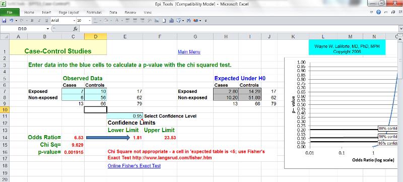
The computation and interpretation of the odds ratio in a case-control study has already been discussed in the modules on Overview of Analytic Studies and Measures of Association. Additionally, one can compute the confidence interval for the odds ratio, and statistical significance can also be evaluated by using a chi-square test (or a Fisher's Exact Test if the sample size is small) to compute a p-value. These calculations can be done using the Case-Control worksheet in the Excel file called EpiTools.XLS.
Advantages:
Disadvantages: