Multivariable Methods

Authors:

Lisa Sullivan, Professor of Biostatistics

Wayne W. LaMorte, MD, PhD, MPH, Professor of Epidemiology

Boston University School of Public Health

Simple Linear Regression

Regression analysis makes use of mathematical models to describe relationships. For example, suppose that height was the only determinant of body weight. If we were to plot height (the independent or 'predictor' variable) as a function of body weight (the dependent or 'outcome' variable), we might see a very linear relationship, as illustrated below.

We could also describe this relationship with the equation for a line, Y = a + b(x), where 'a' is the Y-intercept and 'b' is the slope of the line. We could use the equation to predict weight if we knew an individual's height. In this example, if an individual was 70 inches tall, we would predict his weight to be:

Weight = 80 + 2 x (70) = 220 lbs.

In this simple linear regression, we are examining the impact of one independent variable on the outcome. If height were the only determinant of body weight, we would expect that the points for individual subjects would lie close to the line. However, if there were other factors (independent variables) that influenced body weight besides height (e.g., age, calorie intake, and exercise level), we might expect that the points for individual subjects would be more loosely scattered around the line, since we are only taking height into account.

Multiple Linear Regression Analysis

Multiple linear regression analysis is an extension of simple linear regression analysis which enables us to assess the association between two or more independent variables and a single continuous dependent variable.

This is a very useful procedure for identifying and adjusting for confounding. To provide an intuitive understanding of how multiple linear regression does this, consider the following hypothetical example.

Suppose an investigator had developed a scoring system that enabled her to predict an individual's body mass index (BMI) based on information about what they ate and how much. The investigator wanted to test this new "diet score" to determine how closely it was associated with actual measurements of BMI. Information is collected from a small sample of subjects in order to compute their "diet score," and the weight and height of each subject is measured in order to compute their BMI. The graph below shows the relationship between the new "diet score" and BMI, and it suggests that the "diet score" is not a very good predictor, (i.e., there is little if any association between the two.

While this is discouraging, the investigator considers that it is possible that confounding by age and/or gender is masking the true relationship between "diet score" and BMI. She first identifies which subjects who are older than 20 years old, and it turns out that the younger subjects and older subjects are clustered in the scatter plot, as shown in the figure below.

The investigator suspected that gender might also be a confounding factor, and when she identified males and females, the graph looked like this:

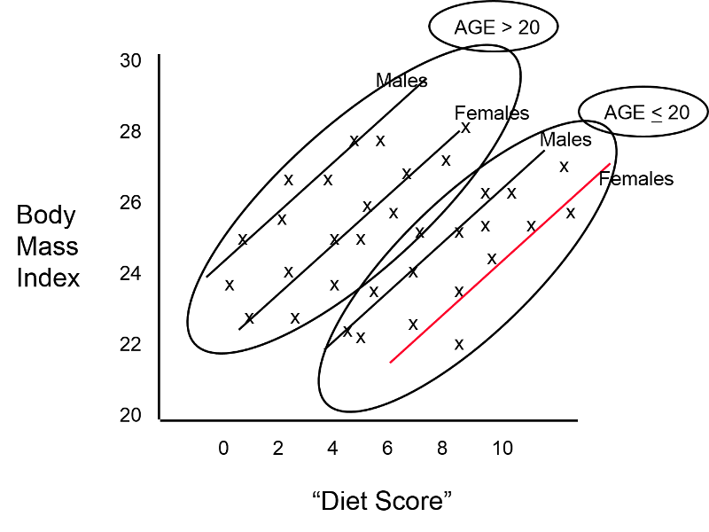
These findings indicate that both age and gender have an impact on BMI, because the older group has higher BMIs than the younger group, while males consistently have higher BMIs than the females. In addition, age and gender are also associated with "diet score," which is the "exposure" of interest, because diet scores are not equally distributed by gender or by age. In other words, both age and gender meet the criteria to be confounders. We can also see (in this very hypothetical example) that there is a striking linear relationship between "diet score" and BMI within each of the four age and gender groups. In other words, it is only after "taking into account" these two confounding variables that we can see that there really is a relationship between diet score and BMI. The true relationship was confounded by these other factors.

When analyzing data, it is always easier to deal with numeric data instead of text. For example, when dealing with dichotomous data the number "1" might conveniently indicate that the characteristic is present instead of "yes" or "true," and the number "0" conveniently indicates "no" or "false". It is also best to organize data sets so that the information for individual subjects is listed in a row, and the columns contain the variables. Consequently, in this scenario my data set would perhaps look something like this:

With data is are coded in this fashion, matrix math can be used to find the coefficients for each variable that led to the best "fit" of the data. For the hypothetical example we are considering here, multiple linear regression analysis could be used to compute the coefficients, and these could be used to describe the relationships in the graph mathematically with the following equation:

BMI = 18.0 + 1.5 (diet score) + 1.6 (male) + 4.2 (age>20)

Note that the numbers in red are the coefficients that the analysis provided.

The Independent Effect of Each Independent Variable

In a sense, the equation above is a prediction of what an individual's BMI will be based on their diet score, gender and age group. The equation has an intercept of 18.0, meaning that I start with a baseline value of 18. I then multiply 1.5 x (diet score); I multiply 1.6 x (male) and multiply 4.2 x (age>20). But remember that in the data base I coded male as 1 for males and as 0 for females; for age group I coded it as 1 if the subject was older than 20 and coded it as 0 if they were less than 20.

Besides being useful for describing the relationships and making predictions, this mathematical description provides a powerful mean of controlling for confounding. For example, the coefficient 1.5 for diet score indicates that for each additional point in diet score, I must add 1.5 units to my prediction, regardless of whether it is a male or female or an adult or a child. In other words, the equation has quantified the association of diet score on BMI independent of (i.e., controlling for) gender and age group. Similarly, it means that I should add 1.6 units to my prediction if the individual is a male, regardless of there age and diet score. And I should add 4.2 to my prediction if the person is over age 20, regardless of their diet score or gender. As a result, the regression analysis has enabled us to dissect out the independent (unconfounded) association of each factor with the outcome of interest. The equation describes the graphical representation of this data, shown below.

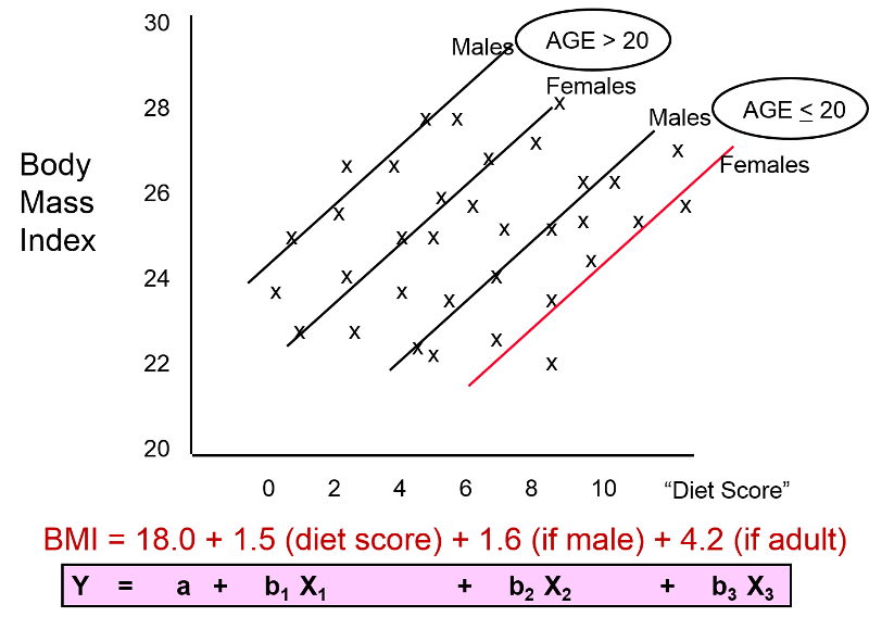
The figure above and the equation enable us to see the impact of each of the independent variables after controlling for confounding. The equation is a mathematical expression of what we see in the figure, and the coefficients for each variable describe an unconfounded measure of the association of each variable with the outcome.

The Multiple Linear Regression Equation

The multiple linear regression equation is as follows:

,

where is the predicted or expected value of the dependent variable, X₁ through X_p are p distinct independent or predictor variables, b₀ is the value of Y when all of the independent variables (X₁ through X_p) are equal to zero, and b₁ through b_p are the estimated regression coefficients. Each regression coefficient represents the change in Y relative to a one unit change in the respective independent variable. In the multiple regression situation, b₁, for example, is the change in Y relative to a one unit change in X₁, holding all other independent variables constant (i.e., when the remaining independent variables are held at the same value or are fixed). Again, statistical tests can be performed to assess whether each regression coefficient is significantly different from zero.

Identifying & Controlling for Confounding With Multiple Linear Regression

As suggested on the previous page, multiple regression analysis can be used to assess whether confounding exists, and, since it allows us to estimate the association between a given independent variable and the outcome holding all other variables constant, multiple linear regression also provides a way of adjusting for (or accounting for) potentially confounding variables that have been included in the model.

Suppose we have a risk factor or an exposure variable, which we denote X₁ (e.g., X₁=obesity or X₁=treatment), and an outcome or dependent variable which we denote Y. We can estimate a simple linear regression equation relating the risk factor (the independent variable) to the dependent variable as follows:

where b₁ is the estimated regression coefficient that quantifies the association between the risk factor and the outcome.

If we now want to assess whether a third variable (e.g., age) is a confounder, we can denote the potential confounder X₂, and then estimate a multiple linear regression equation as follows:

In the multiple linear regression equation, b₁ is the estimated regression coefficient that quantifies the association between the risk factor X₁ and the outcome, adjusted for X₂ (b₂ is the estimated regression coefficient that quantifies the association between the potential confounder and the outcome). As noted earlier, some investigators assess confounding by assessing how much the regression coefficient associated with the risk factor (i.e., the measure of association) changes after adjusting for the potential confounder. In this case, we compare b₁ from the simple linear regression model to b₁ from the multiple linear regression model. As a rule of thumb, if the regression coefficient from the simple linear regression model changes by more than 10%, then X₂ is said to be a confounder.

Once a variable is identified as a confounder, we can then use multiple linear regression analysis to estimate the association between the risk factor and the outcome adjusting for that confounder. The test of significance of the regression coefficient associated with the risk factor can be used to assess whether the association between the risk factor is statistically significant after accounting for one or more confounding variables. This is also illustrated below.

Example:

The Association Between BMI and Systolic Blood Pressure 

Suppose we want to assess the association between BMI and systolic blood pressure using data collected in the seventh examination of the Framingham Offspring Study. A total of n=3,539 participants attended the exam, and their mean systolic blood pressure was 127.3 with a standard deviation of 19.0. The mean BMI in the sample was 28.2 with a standard deviation of 5.3.

A simple linear regression analysis reveals the following:

The simple linear regression model is:

where is the predicted of expected systolic blood pressure. The regression coefficient associated with BMI is 0.67; each one unit increase in BMI is associated with a 0.67 unit increase in systolic blood pressure. The association between BMI and systolic blood pressure is also statistically significant (p=0.0001).

Suppose we now want to assess whether age (a continuous variable, measured in years), male gender (yes/no), and treatment for hypertension (yes/no) are potential confounders, and if so, appropriately account for these using multiple linear regression analysis. For analytic purposes, treatment for hypertension is coded as 1=yes and 0=no. Gender is coded as 1=male and 0=female. A multiple regression analysis reveals the following:

The multiple regression model is:

Notice that the association between BMI and systolic blood pressure is smaller (0.58 versus 0.67) after adjustment for age, gender and treatment for hypertension. BMI remains statistically significantly associated with systolic blood pressure (p=0.0001), but the magnitude of the association is lower after adjustment. The regression coefficient decreases by 13%.

[Note: Some investigators compute the percent change using the adjusted coefficient as the "beginning value," since it is theoretically unconfounded. With this approach the percent change would be = 0.09/0.58 = 15.5%. Both approaches are used, and the results are usually quite similar.]

Using the informal 10% rule (i.e., a change in the coefficient in either direction by 10% or more), we meet the criteria for confounding. Thus, part of the association between BMI and systolic blood pressure is explained by age, gender, and treatment for hypertension.

This suggests a useful way of identifying confounding. Typically, we try to establish the association between a primary risk factor and a given outcome after adjusting for one or more other risk factors. One useful strategy is to use multiple regression models to examine the association between the primary risk factor and the outcome before and after including possible confounding factors. If the inclusion of a possible confounding variable in the model causes the association between the primary risk factor and the outcome to change by 10% or more, then the additional variable is a confounder.

Relative Importance of the Independent Variables 

Assessing only the p-values suggests that these three independent variables are equally statistically significant. The magnitude of the t statistics provides a means to judge relative importance of the independent variables. In this example, age is the most significant independent variable, followed by BMI, treatment for hypertension and then male gender. In fact, male gender does not reach statistical significance (p=0.1133) in the multiple regression model. Some investigators argue that regardless of whether an important variable such as gender reaches statistical significance it should be retained in the model in order to control for possible confounding. Other investigators only retain variables that are statistically significant.

This is yet another example of the complexity involved in multivariable modeling. The multiple regression model produces an estimate of the association between BMI and systolic blood pressure that accounts for differences in systolic blood pressure due to age, gender and treatment for hypertension.

A one unit increase in BMI is associated with a 0.58 unit increase in systolic blood pressure holding age, gender and treatment for hypertension constant. Each additional year of age is associated with a 0.65 unit increase in systolic blood pressure, holding BMI, gender and treatment for hypertension constant.

Men have higher systolic blood pressures, by approximately 0.94 units, holding BMI, age and treatment for hypertension constant and persons on treatment for hypertension have higher systolic blood pressures, by approximately 6.44 units, holding BMI, age and gender constant. The multiple regression equation can be used to estimate systolic blood pressures as a function of a participant's BMI, age, gender and treatment for hypertension status. For example, we can estimate the blood pressure of a 50 year old male, with a BMI of 25 who is not on treatment for hypertension as follows:

We can estimate the blood pressure of a 50 year old female, with a BMI of 25 who is on treatment for hypertension as follows:

Evaluating Effect Modification With Multiple Linear Regression

Considered data from a clinical trial designed to evaluate the efficacy of a new drug to increase HDL cholesterol. One hundred patients enrolled in the study and were randomized to receive either the new drug or a placebo. The investigators were at first disappointed to find very little difference in the mean HDL cholesterol levels of treated and untreated subjects.

However, when they analyzed the data separately in men and women, they found evidence of an effect in men, but not in women. We noted that when the magnitude of association differs at different levels of another variable (in this case gender), it suggests that effect modification is present.

Multiple regression analysis can be used to assess effect modification. This is done by estimating a multiple regression equation relating the outcome of interest (Y) to independent variables representing the treatment assignment, sex and the product of the two (called the treatment by sex interaction variable). For the analysis, we let T = the treatment assignment (1=new drug and 0=placebo), M = male gender (1=yes, 0=no) and TM, i.e., T * M or T x M, the product of treatment and male gender. In this case, the multiple regression analysis revealed the following: 

The multiple regression model is:

The details of the test are not shown here, but note in the table above that in this model, the regression coefficient associated with the interaction term, b₃, is statistically significant (i.e., H₀: b₃ = 0 versus H₁: b₃ ≠ 0). The fact that this is statistically significant indicates that the association between treatment and outcome differs by sex.

The model shown above can be used to estimate the mean HDL levels for men and women who are assigned to the new medication and to the placebo. In order to use the model to generate these estimates, we must recall the coding scheme (i.e., T = 1 indicates new drug, T=0 indicates placebo, M=1 indicates male sex and M=0 indicates female sex).

The expected or predicted HDL for men (M=1) assigned to the new drug (T=1) can be estimated as follows:

The expected HDL for men (M=1) assigned to the placebo (T=0) is:

Similarly, the expected HDL for women (M=0) assigned to the new drug (T=1) is:

The expected HDL for women (M=0)assigned to the placebo (T=0) is:

Notice that the expected HDL levels for men and women on the new drug and on placebo are identical to the means shown the table summarizing the stratified analysis. Because there is effect modification, separate simple linear regression models are estimated to assess the treatment effect in men and women:

 The regression models are:

In Men:

In Women:

In men, the regression coefficient associated with treatment (b₁=6.19) is statistically significant (details not shown), but in women, the regression coefficient associated with treatment (b₁= -0.36) is not statistically significant (details not shown).

Multiple linear regression analysis is a widely applied technique. In this section we showed here how it can be used to assess and account for confounding and to assess effect modification. The techniques we described can be extended to adjust for several confounders simultaneously and to investigate more complex effect modification (e.g., three-way statistical interactions).

There is an important distinction between confounding and effect modification. Confounding is a distortion of an estimated association caused by an unequal distribution of another risk factor. When there is confounding, we would like to account for it (or adjust for it) in order to estimate the association without distortion. In contrast, effect modification is a biological phenomenon in which the magnitude of association is differs at different levels of another factor, e.g., a drug that has an effect on men, but not in women. In the example, present above it would be in inappropriate to pool the results in men and women. Instead, the goal should be to describe effect modification and report the different effects separately.

There are many other applications of multiple regression analysis. A popular application is to assess the relationships between several predictor variables simultaneously, and a single, continuous outcome. For example, it may be of interest to determine which predictors, in a relatively large set of candidate predictors, are most important or most strongly associated with an outcome. It is always important in statistical analysis, particularly in the multivariable arena, that statistical modeling is guided by biologically plausible associations.

"Dummy" Variables in Regression Models 

Independent variables in regression models can be continuous or dichotomous. Regression models can also accommodate categorical independent variables. For example, it might be of interest to assess whether there is a difference in total cholesterol by race/ethnicity. The module on Hypothesis Testing presented analysis of variance as one way of testing for differences in means of a continuous outcome among several comparison groups. Regression analysis can also be used. However, the investigator must create indicator variables to represent the different comparison groups (e.g., different racial/ethnic groups). The set of indicator variables (also called dummy variables) are considered in the multiple regression model simultaneously as a set independent variables.

For example, suppose that participants indicate which of the following best represents their race/ethnicity: White, Black or African American, American Indian or Alaskan Native, Asian, Native Hawaiian or Pacific Islander or Other Race. This categorical variable has 6 response options. To consider race/ethnicity as a predictor in a regression model, we create five indicator variables (one less than the total number of response options) to represent the 6 different groups. To create the set of indicators, or set of dummy variables, we first decide on a reference group or category. In this example, the reference group is the racial group that we will compare the other groups against. Indicator variable are created for the remaining groups are coded 1 for participants who are in that group (e.g., are of the specific race/ethnicity of interest), and all others are coded 0. In the multiple regression model, the regression coefficients associated with each of the dummy variables (representing in this example each race/ethnicity group) are interpreted as the expected difference in the mean of the outcome variable for that race/ethnicity as compared to the reference group, holding all other predictors constant. The example below uses an investigation of risk factors for low birth weight to illustrates this technique as well as the interpretation of the regression coefficients in the model.

Example of the Use of Dummy Variables

An observational study is conducted to investigate risk factors associated with infant birth weight. The study involves 832 pregnant women. Each woman provides demographic and clinical data and is followed through the outcome of pregnancy. At the time of delivery, the infant s birth weight (grams) is measures, as is their gestational age (weeks). Birth weights vary widely and range from 404 to 5400 grams. The mean birth weight is 3367.83 grams with a standard deviation of 537.21 grams. Investigators wish to determine whether there are differences in birth weight by infant gender, gestational age, mother's age and mother's race. In the study sample, 421/832 (50.6%) of the infants are male and the mean gestational age at birth is 39.49 weeks with a standard deviation of 1.81 weeks (range 22-43 weeks). The mean mother's age is 30.83 years with a standard deviation of 5.76 years (range 17-45 years). Approximately 49% of the mothers are white; 41% are Hispanic; 5% are black; and 5% identify themselves as other race. A multiple regression analysis is performed relating infant gender (coded 1=male, 0=female), gestational age in weeks, mother's age in years and 3 dummy or indicator variables reflecting mother's race. The results are summarized in the table below.

Many of the predictor variables are statistically significantly associated with birth weight. Male infants are approximately 175 grams heavier than female infants, adjusting for gestational age, mother's age and mother's race/ethnicity. Gestational age is highly significant (p=0.0001), with each additional gestational week associated with an increase of 179.89 grams in birth weight, holding infant gender, mother's age and mother's race/ethnicity constant. Mother's age does not reach statistical significance (p=0.6361). Mother's race is modeled as a set of three dummy or indicator variables. In this analysis, white race is the reference group. Infants born to black mothers have lower birth weight by approximately 140 grams (as compared to infants born to white mothers), adjusting for gestational age, infant gender and mothers age. This difference is marginally significant (p=0.0535). There are no statistically significant differences in birth weight in infants born to Hispanic versus white mothers or to women who identify themselves as other race as compared to white.

Multiple Logistic Regression Analysis

Introduction to Logistic Regression Analysis

Logistic regression analysis is a popular and widely used analysis that is similar to linear regression analysis except that the outcome is dichotomous (e.g., success/failure, or yes/no, or died/lived).

The earlier discussion in this module provided a demonstration of how regression analysis can provide control of confounding for multiple factors simultaneously when evaluating continuously distributed outcome variables like body weight or BMI (i.e., outcomes that can be measured as an infinite number of values). However, some outcomes are dichotomous, i.e. they either occurred or they didn't. For example, the subjects either died or didn't; the subjects either developed obesity or they didn't. In these situations, it is desirable to utilize a similar approach to adjust for multiple possible confounding factors simultaneously, but multiple linear regression can't be used since the outcome is all or none. This situation is dealt with be utilizing an analogous method called multiple logistic regression.

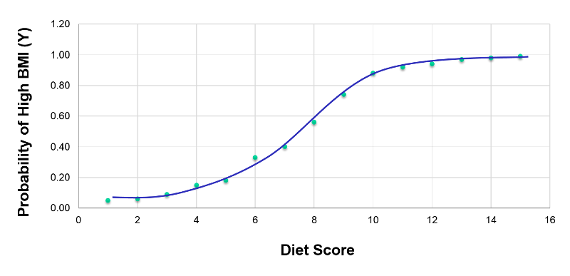
Consider again the example looking at the association between diet score and BMI, but now let's make the outcome dichotomous by arbitrarily categorizing each BMI as either "high" or "low". Our goal now is to create a mathematical model that evaluates the likelihood of "high" BMI. We can begin by summarizing the results as shown below. For any given diet score, we compute the probability of having a high BMI as shown in the last column.

If we were to plot the probability of having a high BMI at any given diet score, it would look like the graph below, with a distinctive sigmoidal shape.

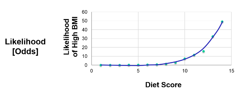
This transformation of the dependent variable into a probability is helpful in limiting the dependent variable to values between 0 and 1, but it isn't linear. Nevertheless, we can perform additional transformations. From the same data we could also plot the odds or the "likelihood" of having a high BMI at each diet score, where the likelihood (odds) = (probability of the outcome occurring) divided by (probability of the outcome not occurring). This is shown in the graph elow.

If we take the natural logarithm of the odds of a high BMI and plot this as a function of diet score, we get the linear graph below.

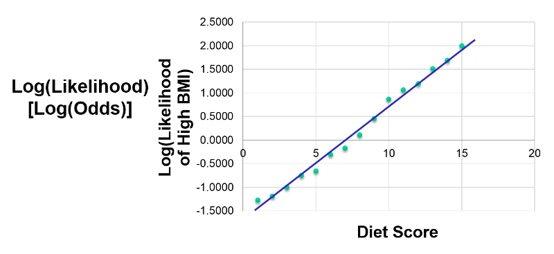
Since this is linear, we can treat this like a multiple linear; this is what logistic regression does. By taking the natural log, I have linearized this relationship, so now I can perform a regression analysis, just as I did for multiple linear regression. This makes it possible to examine how the log(odds of the outcome) is associated with multiple independent risk factors such as diet score, age group, and male gender. The model for evaluating these relationships could be summarized in the figure below.

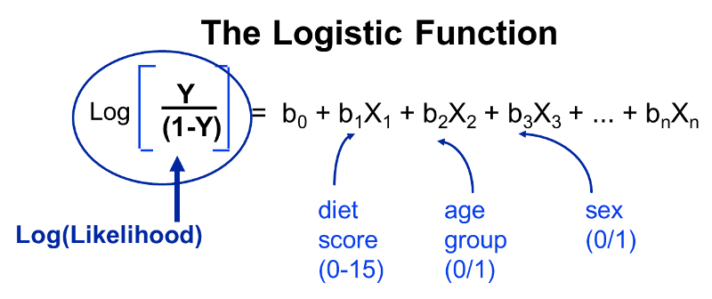
Note that the outcome (the dependent variable) is dichotomous - it either occurred or it didn't. In essence, we examine the odds of an outcome occurring (or not), and by using the natural log of the odds of the outcome as the dependent variable the relationships can be linearized and analyzed using methods analogous to those used in multiple linear regression analysis.

Note that the outcome (dependent variable) always dichotomous in logistic regression, but the independent variables (i.e., the predictor variables) may be either dichotomous or continuously distributed measurements (just as in multiple linear regression). Therefore, I could include the following independent variables:

• Diet Score (measurement from 0-15),
• ADULT (1 if age>20; 0 if younger)
• MALE (1 if male; 0 if female)

Logistic Regression Analysis

The outcome in logistic regression analysis is often coded as 0 or 1, where 1 indicates that the outcome of interest is present, and 0 indicates that the outcome of interest is absent. If we define p as the probability that the outcome is 1, the multiple logistic regression model can be written as follows:

is the expected probability that the outcome is present; X₁ through X_p are distinct independent variables; and b₀ through b_p are the regression coefficients. The multiple logistic regression model is sometimes written differently. In the following form, the outcome is the expected log of the odds that the outcome is present,

Notice that the right hand side of the equation above looks like the multiple linear regression equation. However, the technique for estimating the regression coefficients in a logistic regression model is different from that used to estimate the regression coefficients in a multiple linear regression model. In logistic regression the coefficients derived from the model (e.g., b₁) indicate the change in the expected log odds relative to a one unit change in X₁, holding all other predictors constant. Therefore, the antilog of an estimated regression coefficient, exp(b_i), produces an odds ratio, as illustrated in the example below.

Example of Logistic Regression - Association Between Obesity and CVD

We previously analyzed data from a study designed to assess the association between obesity (defined as BMI > 30) and incident cardiovascular disease. Data were collected from participants who were between the ages of 35 and 65, and free of cardiovascular disease (CVD) at baseline. Each participant was followed for 10 years for the development of cardiovascular disease. A summary of the data can be found on page 2 of this module. The unadjusted or crude relative risk was RR = 1.78, and the unadjusted or crude odds ratio was OR =1.93. We also determined that age was a confounder, and using the Cochran-Mantel-Haenszel method, we estimated an adjusted relative risk of RR_CMH =1.44 and an adjusted odds ratio of OR_CMH =1.52. We will now use logistic regression analysis to assess the association between obesity and incident cardiovascular disease adjusting for age.

 The logistic regression analysis reveals the following: 

The simple logistic regression model relates obesity to the log odds of incident CVD:

Obesity is an indicator variable in the model, coded as follows: 1=obese and 0=not obese. The log odds of incident CVD is 0.658 times higher in persons who are obese as compared to not obese. If we take the antilog of the regression coefficient, exp(0.658) = 1.93, we get the crude or unadjusted odds ratio. The odds of developing CVD are 1.93 times higher among obese persons as compared to non obese persons. The association between obesity and incident CVD is statistically significant (p=0.0017). Notice that the test statistics to assess the significance of the regression parameters in logistic regression analysis are based on chi-square statistics, as opposed to t statistics as was the case with linear regression analysis. This is because a different estimation technique, called maximum likelihood estimation, is used to estimate the regression parameters (See Hosmer and Lemeshow³ for technical details).

Many statistical computing packages also generate odds ratios as well as 95% confidence intervals for the odds ratios as part of their logistic regression analysis procedure. In this example, the estimate of the odds ratio is 1.93 and the 95% confidence interval is (1.281, 2.913).

When examining the association between obesity and CVD, we previously determined that age was a confounder.The following multiple logistic regression model estimates the association between obesity and incident CVD, adjusting for age. In the model we again consider two age groups (less than 50 years of age and 50 years of age and older). For the analysis, age group is coded as follows: 1=50 years of age and older and 0=less than 50 years of age.

 If we take the antilog of the regression coefficient associated with obesity, exp(0.415) = 1.52 we get the odds ratio adjusted for age. The odds of developing CVD are 1.52 times higher among obese persons as compared to non obese persons, adjusting for age. In Section 9.2 we used the Cochran-Mantel-Haenszel method to generate an odds ratio adjusted for age and found the following:

This illustrates how multiple logistic regression analysis can be used to account for confounding. The models can be extended to account for several confounding variables simultaneously. Multiple logistic regression analysis can also be used to assess confounding and effect modification, and the approaches are identical to those used in multiple linear regression analysis. Multiple logistic regression analysis can also be used to examine the impact of multiple risk factors (as opposed to focusing on a single risk factor) on a dichotomous outcome.

Example - Risk Factors Associated With Low Infant Birth Weight

Suppose that investigators are also concerned with adverse pregnancy outcomes including gestational diabetes, pre-eclampsia (i.e., pregnancy-induced hypertension) and pre-term labor. Recall that the study involved 832 pregnant women who provide demographic and clinical data. In the study sample, 22 (2.7%) women develop pre-eclampsia, 35 (4.2%) develop gestational diabetes and 40 (4.8%) develop pre term labor. Suppose we wish to assess whether there are differences in each of these adverse pregnancy outcomes by race/ethnicity, adjusted for maternal age. Three separate logistic regression analyses were conducted relating each outcome, considered separately, to the 3 dummy or indicators variables reflecting mothers race and mother's age, in years. The results are below. 

The only statistically significant difference in pre-eclampsia is between black and white mothers.

Black mothers are nearly 9 times more likely to develop pre-eclampsia than white mothers, adjusted for maternal age. The 95% confidence interval for the odds ratio comparing black versus white women who develop pre-eclampsia is very wide (2.673 to 29.949). This is due to the fact that there are a small number of outcome events (only 22 women develop pre-eclampsia in the total sample) and a small number of women of black race in the study. Thus, this association should be interpreted with caution.

While the odds ratio is statistically significant, the confidence interval suggests that the magnitude of the effect could be anywhere from a 2.6-fold increase to a 29.9-fold increase. A larger study is needed to generate a more precise estimate of effect.

  With regard to gestational diabetes, there are statistically significant differences between black and white mothers (p=0.0099) and between mothers who identify themselves as other race as compared to white (p=0.0150), adjusted for mother's age. Mother's age is also statistically significant (p=0.0378), with older women more likely to develop gestational diabetes, adjusted for race/ethnicity.

With regard to pre term labor, the only statistically significant difference is between Hispanic and white mothers (p=0.0021). Hispanic mothers are 80% less likely to develop pre term labor than white mothers (odds ratio = 0.209), adjusted for mother's age.

Summary

Multivariable methods are computationally complex and generally require the use of a statistical computing package. Multivariable methods can be used to assess and adjust for confounding, to determine whether there is effect modification, or to assess the relationships of several exposure or risk factors on an outcome simultaneously. Multivariable analyses are complex, and should always be planned to reflect biologically plausible relationships. While it is relatively easy to consider an additional variable in a multiple linear or multiple logistic regression model, only variables that are clinically meaningful should be included.

It is important to remember that multivariable models can only adjust or account for differences in confounding variables that were measured in the study. In addition, multivariable models should only be used to account for confounding when there is some overlap in the distribution of the confounder each of the risk factor groups.

Stratified analyses are very informative, but if the samples in specific strata are too small, the analyses may lack precision. In planning studies, investigators must pay careful attention to potential effect modifiers. If there is a suspicion that an association between an exposure or risk factor is different in specific groups, then the study must be designed to ensure sufficient numbers of participants in each of those groups. Sample size formulas must be used to determine the numbers of subjects required in each stratum to ensure adequate precision or power in the analysis. 

References

1. Kleinbaum D, Kupper LL, Muller KE. Applied Regression Analysis and Other Multivariable Methods. PWS-Kent, Boston, MA, 2nd edition, 1988.
2. Jewell NP. Statistics for Epidemiology. New York, NY: Chapman and Hall/CRC. 2004.
3. Hosmer D, Lemeshow S. Applied Logistic Regression. New York: NY: John Wiley & Sons, Inc. 1989.
4. Anderson M, Wilson PW, Odell PM, Kannell WB. An updated coronary risk profile: A statement for health professionals. Circulation. 1991; 83: 356-362.
5. Wilson PWF, D'Agostino RB, Levy D, Belanger AM, Silbershatz H, Kannel WB. Prediction of coronary heart disease using risk factor categories. Circulation. 1998; 97: 1837-1847.
6. SAS version 9.1© 2002-2003 by SAS Institute, Inc., Cary, NC.
7. Aschengrau A, Seage GR. Essentials of Epidemiology for Public Health. Sudbury, MA: Jones and Bartlett Publishers, Inc., 2006.
8. Goldberg JI, Borgen PI. Breast cancer susceptibility testing: Past, present and future. Expert Review of Anticancer Therapy. 2006; 6(8): 1205-1214.
9. Meigs JB, Hu FB, Rifai N, Manson J. Biomarkers of endothelial dysfunction and risk of Type 2 Diabetes Mellitus. Journal of the American Medical Association. 2004; 291: 1978-1986.
10. Stern MP, Williams K, Haffner S. Identification of persons at high risk for Type 2 Diabetes Mellitus: Do we need the oral glucose tolerance test? Annals of Internal Medicine. 2002; 136(8): 575-581.