Confounding and Effect Measure Modification

Authors:

Wayne W. LaMorte, MD, PhD, MPH, Professor of Epidemiology

Lisa Sullivan, PhD, Professor of Biostatistics

Boston University School of Publich Health

NOTE: This module is used for both BS704 and EP713.

Introduction

Confounding is a distortion of the association between an exposure and an outcome that occurs when the study groups differ with respect to other factors that influence the outcome. Unlike selection and information bias, which can be introduced by the investigator or by the subjects, confounding is a type of bias that can be adjusted for in the analysis, provided that the investigators have information on the status of study subjects with respect to potential confounding factors.

Effect modification is distinct from confounding; it occurs when the magnitude of the effect of the primary exposure on an outcome (i.e., the association) differs depending on the level of a third variable. 

Learning Objectives

After completing this module, the student will be able to:

1. Explain the three key properties of a confounder
2. Define and identify confounding
3. Identify three ways to control confounding in the design phase of a study, and identify the strengths and weaknesses of each approach
4. Describe ways to control for confounding in the analysis phase of a study
5. Explain and calculate crude and stratum-specific measures of association
6. Compare crude and adjusted measures of association to identify whether confounding is present and characterize the direction and magnitude of confounding
7. Describe residual confounding and identify possible sources
8. Define and provide an example of effect modification

What is Confounding?

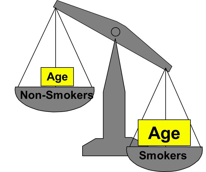
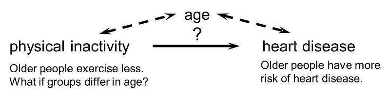
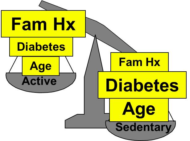
Confounding is a distortion (inaccuracy) in the estimated measure of association that occurs when the primary exposure of interest is mixed up with some other factor that is associated with the outcome. In the diagram below, the primary goal is to ascertain the strength of association between physical inactivity and heart disease. Age is a confounding factor because it is associated with the exposure (meaning that older people are more likely to be inactive), and it is also associated with the outcome (because older people are at greater risk of developing heart disease).

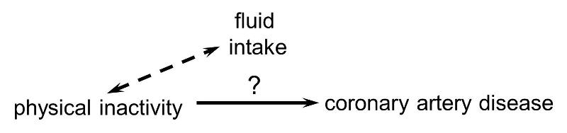
In order for confounding to occur, the extraneous factor must be associated with both the primary exposure of interest and the disease outcome of interest. For example, subjects who are physically active may drink more fluids (e.g., water and sports drinks) than inactive people, but drinking more fluid has no effect on the risk of heart disease, so fluid intake is not a confounding factor here.

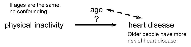
Or, if the age distribution is similar in the exposure groups being compared, then age will not cause confounding.

Refining Our Understanding of Confounding

Rothman and others use a study by Stark and Mantel to illustrate the key features of confounding. These authors investigated the association between birth order and the risk of Down syndrome. The first graph to the right shows a clear trend toward increasing prevalence of Down syndrome with increasing birth order, or an association between increasing birth order and risk of Down syndrome.

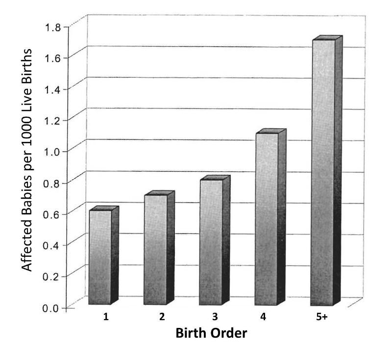
A 5th born child appears to have roughly a 4-fold increase in risk of being born with Down syndrome. Results like this also invite us to think about the mechanisms by which this occurred. Why might birth order cause a greater risk of Down syndrome? Keep in mind that this analysis does not consider any other "risk factors" besides birth order.

However, consider also that the order in which a women's children are born is also linked to her age at the time of her child's birth. When Stark and Mantel examined the relationship between maternal age at birth and risk of the child having Down syndrome, they observed the relationship depicted in the bar graph below. This shows an even more striking relationship between maternal age at birth and the child's risk of being born with Down syndrome.

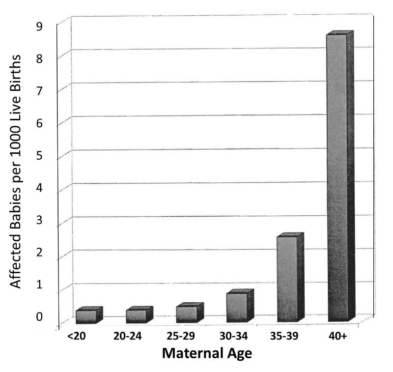
Obviously, women giving birth to their fifth child are on average, older than women giving birth to their first child. In other words, birth order of children is mixed up with maternal age when a child is born. The correlation between maternal age and prevalence of Down syndrome is much stronger than the correlation with birth order, and a woman having her 5th child is clearly older than when she gave birth to her previous children. In view of this, the relationship between birth order and prevalence of Down syndrome is confounded by age. In other words, the association between birth order and Down syndrome is exaggerated by the confounding effect of maternal age.

But is the converse also true? Is the effect of maternal age confounded by birth order? It is possible, but only if birth order really has some independent effect on the likelihood of Down syndrome, i.e. an effect independent of the fact that birth order is linked to maternal age. Rothman points out that a good way to sort this out is to look at both effects simultaneously, as in the graph below.

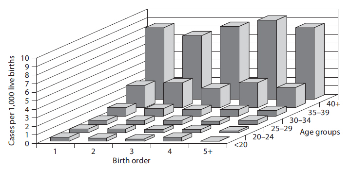
In a sense this graph shows the relationships by stratifying the prevalence of Down syndrome by both birth order and maternal age. If one focuses on how prevalence changes within any particular maternal age group looking from side to side, it is clear that increasing birth order does not correlate with the prevalence of Down syndrome. In other words, if one "controls for maternal age," there is no evidence that birth order has any impact. On the other hand, if one now examines changes in prevalence within each of the birth order groups by looking from front to back within a given birth order, there is clearly a marked increase in prevalence as maternal age increases within all five levels of birth order. In other words, even after taking birth order into account (i.e., controlling for birth order) the strong association with maternal age persists.

Based on this analysis one can conclude that the association between birth order and Down syndrome was confounded by age. The different birth order groups had different age distributions, and maternal age is clearly associated with prevalence of Down syndrome. As a result, the apparent association between birth order and and Down syndrome that was seen in the first figure was completely due to the confounding effect of age. On the other hand, the association between maternal age and Down syndrome was NOT confounded by birth order, because birth order has no impact on the prevalence of Down syndrome, and the association between age and Down was not distorted by differences in birth order. 

Unraveling the Complexity of Health Problems

Most health problems have many determinants ("risk factors"), so it is not surprising that there is a lot of potential for confounding. While this can represent a barrier to testing a particular hypothesis, it is also an opportunity to dissect the many determinants and to define their relative importance.

Conditions Necessary for Confounding

There are three conditions that must be present for confounding to occur:

1. The confounding factor must be associated with both the risk factor of interest and the outcome.
2. The confounding factor must be distributed unequally among the groups being compared.
3. A confounder cannot be an intermediary step in the causal pathway from the exposure of interest to the outcome of interest.

For example, it is known that modest alcohol consumption is associated with a decreased risk of coronary heart disease, and it is believed that one of the mechanisms by which alcohol causes a reduced risk is that alcohol raises blood levels of HDL, the so called "good cholesterol." Higher levels of HDL are known to be associated with a reduced risk of heart disease. Consequently it is believed that modest alcohol consumption raises HDL levels, and this, in turn, reduces coronary heart disease. In a situation like this HDL levels are not confounder of the association between alcohol and heart disease, because it is part of the mechanism by which alcohol produces this beneficial effect. If increased HDL is a consequence of alcohol consumption and part of the mechanism by which it lowers the risk of heart disease, then it is not a confounder..

Not surprisingly, since most diseases have multiple contributing causes (risk factors), there are many possible confounders.

• A confounder can be another risk factor for the disease. For example, in the hypothetical cohort study testing the association between exercise and heart disease, age is a confounder because it is a risk factor for heart disease.
• Similarly a confounder can also be a preventive factor for the disease. If those people who exercised regularly were more likely to take aspirin, and aspirin reduces the risk of heart disease, then aspirin use would be a confounding factor that would tend to exaggerate the benefit of exercise.
• A confounder can also be a surrogate or a marker for some other cause of disease. For example, socioeconomic status may be a confounder in this example because lower socioeconomic status is a marker for a complex set of poorly understood factors that seem to carry a higher risk of heart disease.

As a result, there may be many possible confounding factors that could influence an association. For example, in looking at the association between exercise and heart disease, other possible confounders might include age, diet, smoking status and a variety of other risk factors that might be unevenly distributed between the groups being compared.

Aside from their physical inactivity, sedentary subjects may be more likely to smoke, to have high blood pressure and diabetes, and to consume diets with a higher fat content; all of these factors would tend to increase the risk of coronary heart disease. On the other hand, subjects who go to a gym regularly (active) may be more likely to be males and perhaps more likely to have a family history of heart disease, i.e., factors that might increase the risk of active subjects. Consequently, there may be many confounders that can distort the estimate of association in one direction or another.

Identifying Confounding

1. A simple, direct way to determine whether a given risk factor caused confounding is to compare the estimated measure of association before and after adjusting for confounding. In other words, compute the measure of association both before and after adjusting for a potential confounding factor. If the difference between the two measures of association is 10% or more, then confounding was present. If it is less than 10%, then there was little, if any, confounding. How to do this will be addressed in greater detail below.
2. Other investigators will determine whether a potential confounding variable is associated with the exposure of interest and whether it is associated with the outcome of interest. If there is a clinically meaningful relationship between an the variable and the risk factor and between the variable and the outcome (regardless of whether that relationship reaches statistical significance), the variable is regarded as a confounder.
3. Still other investigators perform formal tests of hypothesis to assess whether the variable is associated with the exposure of interest and with the outcome.

Effects of Confounding

• May account for all or part of an apparent association.
• May cause an overestimate of the true association (positive confounding) or an underestimate of the association (negative confounding).

The magnitude confounding can be quantified by computing the percentage difference between the crude and adjusted measures of effect. There are two slightly different methods that investigators use to compute this, as illustrated below.

Percent difference is calculated by calculating the difference between the starting value and ending value and then dividing this by the starting value. Many investigators consider the crude measure of association to be the "starting value".

• Method Favored by Biostatisticians

Other investigators consider the adjusted measure of association to be the starting value, because it is less confounded than the crude measure of association.

• Method Favored by Epidemiologists

While the two methods above differ slightly, they generally produce similar results and provide a reasonable way of assessing the magnitude of confounding. Note also that confounding can be negative or positive in value.

Residual Confounding, Confounding by Indication, & Reverse Causality

Residual Confounding

Residual confounding is the distortion that remains after controlling for confounding in the design and/or analysis of a study. There are three causes of residual confounding:

1. There were additional confounding factors that were not considered, or there was no attempt to adjust for them, because data on these factors was not collected.
2. Control of confounding was not tight enough. For example, a study of the association between physical activity and age might control for confounding by age by a) restricting the study population to subject between the ages of 30-80 or b) matching subjects by age within 20 year categories. In either event there might be persistent differences in age among the groups being compared. Residual differences in confounding might also occur in a randomized clinical trial if the sample size was small. In a stratified analysis or in a regression analysis there could be residual confounding because data on confounding variable was not precise enough, e.g., age was simply classified as "young" or "old".
3. There were many errors in the classification of subjects with respect to confounding variables.

Confounding by Indication

Confounding by indication is a special type of confounding that can occur in observational (non-experimental) pharmaco-epidemiologic studies of the effects and side effects of drugs. This type of confounding arises from the fact that individuals who are prescribed a medication or who take a given medication are inherently different from those who do not take the drug, because they are taking the drug for a reason. In medical terminology, such individuals have an "indication" for use of the drug. Even if the study population consists of subjects with the same disease, e.g., osteoarthritis, they may differ in the severity of their disease and may therefore differ in the need for medication. Aschengrau and Seage give the example of studies of the association between antidepressant drug use and infertility. The use of antidepressant medications may appear to be associated with an increased risk of infertility. However, depression itself is a known risk factor for infertility. As a result, there would appear to be an association between antidepressants and infertility. One way of dealing with this is to study the association in subjects who are receiving different treatments for the same underlying disease condition.

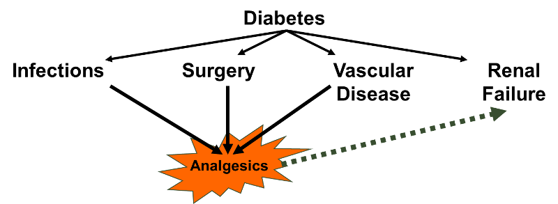
A variation on this might be dubbed "confounding by contraindication." For example, in the case-control study by Perneger and Whelton examining the association between analgesic drug use and kidney failure the authors compared prior analgesic use between patients receiving kidney dialysis and population controls without known kidney disease. Suppose that patients on dialysis had been advised to avoid taking aspirin because of its effects on blood clotting; they may have been advised to take acetaminophen (Tylenol) instead). If the group of dialysis cases included a number of people who had been on long-term dialysis, this would result in a decreased frequency of aspirin use and and increased use of Tylenol in the case group. As a result, an association with aspirin would be underestimated, while an association with Tylenol would be overestimated.

Reverse Causality

Reverse causality occurs when the probability of the outcome is causally related to the exposure being studied. For example, Child feeding recommendations of the World Health Organization include breastfeeding for two years or more, because of evidence that breast fed children have a reduced risk of infectious agents and are less likely to die. However, some studies have produced conflicting concerns. One possibility is that in communities with very poor resources the children who are at greatest risk and perhaps have the least access to other food sources are more likely to be breast fed for at least two years. A comparison of growth and development between these children and more advantaged children would likely find less progress in the breast fed group. (See "Association of Breastfeeding and Stunting in Peruvian Toddlers: An Example of Reverse Causality" by Marquis GS, et al.: International Journal of Epidemiology 1997; 26: 349–356.

The case-control study by Perneger and Whelton may also have been affected by reverse causality. Diabetes is a leading cause of renal failure in the US, and chronic diabetes is associated with a number of other health problems such as cardiovascular diseases and infections that could result in a greater use of analgesics. If so, the dialysis cases whose renal failure resulted from diabetes might have taken more analgesics because of their diabetes. Nevertheless, it would appear that analgesic use was associated with an increased risk of renal failure rather than vice versa.

Control of Confounding in Study Design

Restriction

One of the conditions necessary for confounding to occur is that the confounding factor must be distributed unequally among the groups being compared. Consequently, one of the strategies employed for avoiding confounding is to restrict admission into the study to a group of subjects who have the same levels of the confounding factors. For example, in the hypothetical study looking at the association between physical activity and heart disease, suppose that age and gender were the only two confounders of concern. If so, confounding by these factors could have been avoided by making sure that all subjects were males between the ages of 40-50. This will ensure that the age distributions are similar in the groups being compared, so that confounding will be minimized.

This approach to controlling confounding is simple and effective, but it has several limitations:

• It reduces the number of subjects who are eligible (may cause sample size problem).
• Residual confounding can occur if you don't restrict narrowly enough. For example, in the study on exercise and heart disease, the investigators might have restricted the study to men aged 40-65. However, the age-related risk of heart disease still varies widely within this range as do levels of physical activity.
• You can't evaluate the effects of factors that have been restricted for. For example, if the study is limited to men aged 45-50, you can't use this study to examine the effects of gender or age (because these factors don't vary within your sample).
• Restriction limits generalizability. For example, if you restrict the study to men, you may not be able to generalize the findings to women.

Matching

Instead of restriction, one could also ensure that the study groups do not differ with respect to possible confounders such as age and gender by matching the two comparison groups. For example, for every active male between the ages of 40-50, we could find and enroll an inactive male between the ages of 40-50. In this way, the groups we are comparing can artificially be made similar with respect to these factors, so they cannot confound the relationship. This method actually requires the investigators to control confounding in both the design and analysis phases of the study, because the analysis of matched study groups differs from that of unmatched studies. Like restriction, this approach is straightforward, and it can be effective. However, it has the following disadvantages:

• It can be time-consuming and expensive.
• It limits sample size.
• You can't evaluate the effect of the factors you that you matched for.

Nevertheless, matching is useful in the following circumstances:

• When one needs to control for complex, multifaceted variables (e.g., heredity, environmental factors)
• When doing a case-control study in which there are many possible controls, but a smaller number of cases (e.g., 4:1 matching in the study examining the association between DES and vaginal cancer)

Randomization in Clinical Trials

You previously studied randomization in the online module on Clinical Trials. Given the more detailed discussion in this current module of the conditions necessary for confounding to occur, it should be obvious why randomization is such a powerful method to control prevent confounding. If a large number of subjects are allocated to treatment groups by a random method that gives an equal chance of being in any treatment group, then it is likely that the groups will have similar distributions of age, gender, behaviors, and virtually all other known and as yet unknown possible confounding factors. Moreover, the investigators can get a sense of whether randomization has successfully created comparability among the groups by comparing their baseline characteristics.

Control of Confounding in the Analysis - Stratified Analysis

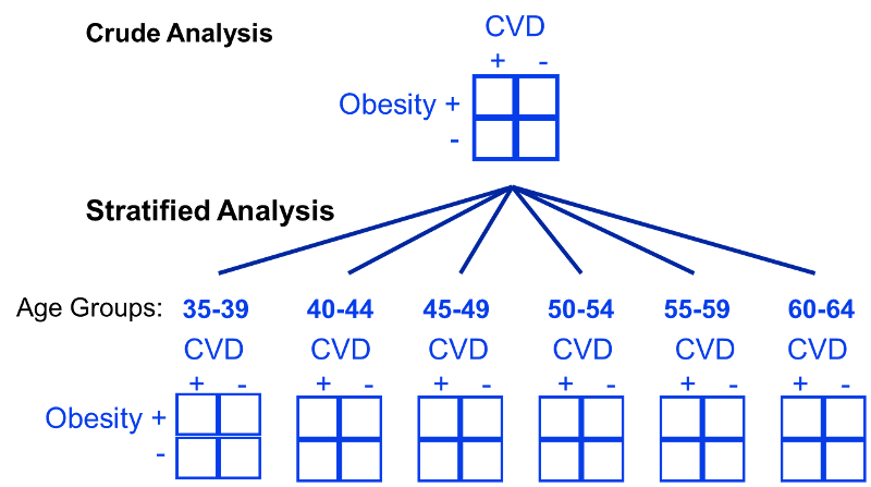
One way of identifying confounding is to examine the primary association of interest at different levels of a potential confounding factor. The side by side tables below examine the relationship between obesity and incident CVD in persons less than 50 years of age and in persons 50 years of age and older, separately. 

Table of Obesity and Incident Cardiovascular Disease by Age Group

The stratum-specific risk ratios are as follows:

• Among those ‹50, the risk ratio is:

• Among those ≥ 50, the risk ratio is:

Recall that the risk ratio for the total, combined sample was RR = 1.79; this is sometimes referred to as the "crude" measure of association, because it is not adjusted for potential confounding factors. The risk ratios for the age-stratified analysis are similar (RR = 1.43 and 1.44, respectively), but less than the crude risk ratio. This indicates that there was confounding by age in the overall sample. We saw that obese subjects were more likely to be 50 and older, and we also saw that those over age 50 had a greater risk of CVD. As a result, the crude analysis overestimated the true association between obesity (per se) and CVD, because of the greater proportion of older subjects among the obese group.

Several things are noteworthy in this example. First, if you compare the cumulative incidence in young versus old active subjects, you can see that older subjects had a higher risk of CVD than younger subjects; this was true for both obese and non-obese subjects. Therefore, age and CVD (the outcome of interest) are associated. In addition, obesity was more common in older subjects, meaning that age and obesity were also associated. Finally, there is no reason to think that age is an intermediary variable in the causal chain between obesity and CVD. Therefore, these observations satisfy all three of the requirements for a confounder.

Comparing the crude and stratum-specific measures of association is a very practical way to determine whether confounding is present and how bad it is. You calculate an overall crude (unadjusted) relative risk (or odds ratio) and compare it to the stratum-specific relative risks (or odds ratios). If the stratum-specific measures of association are similar to the crude measure of association, then there is no confounding by that factor, and you can just use the crude measure of association. However, if the stratified estimates of association differ from the unadjusted estimate by 10% or more, then there is evidence of confounding.

The Cochran-Mantel-Haenszel Method

In the example above we saw that the relationship between obesity and CVD was confounded by age. When the data was pooled, it appeared that the risk ratio for the association between obesity and CVD was 1.79. However, when we stratified the analysis into those age <50 and those age 50+, we saw that both groups had a risk ratio of about 1.43. The distortion was due to the fact that obese individuals tended to be older, and older age is a risk factor for CVD. Consequently, in the analysis using the combined data set, the obese group had the added burden of an additional risk factor.

The Cochran-Mantel-Haenszel method is a technique that generates an estimate of an association between an exposure and an outcome after adjusting for or taking into account confounding. The method is used with a dichotomous outcome variable and a dichotomous risk factor. We stratify the data into two or more levels of the confounding factor (as we did in the example above). In essence, we create a series of two-by-two tables showing the association between the risk factor and outcome at two or more levels of the confounding factor, and we then compute a weighted average of the risk ratios or odds ratios across the strata (i.e., across subgroups or levels of the confounder).

Data Layout for Cochran-Mantel-Haenszel Estimates

Before computing a Cochran-Mantel-Haenszel Estimate, it is important to have a standard layout for the two by two tables in each stratum. We will use the general format depicted here:

Using the notation in this table estimates for a risk ratio or an odds ratio would be computed as follows:

• Risk Ratio:

• Odds Ratio:

Cochran-Mantel-Haenszel Equations

To explore and adjust for confounding, we can use a stratified analysis in which we set up a series of two-by-two tables, one for each stratum (category) of the confounding variable. Having done that, we can compute a weighted average of the estimates of the risk ratios or odds ratios across the strata. The weighted average provides a measure of association that is adjusted for confounding. The weighted averages for risk ratios and odds ratios are computed as follows:

• Cochran-Mantel-Haenszel Estimate for a Risk Ratio

• Cochran-Mantel-Haenszel Estimate for an Odds Ratio

Where a_i, b_i, c_i, and d_i are the numbers of participants in the cells of the two-by-two table in the i^th stratum of the confounding variable, and n_i represents the number of participants in the i^th stratum.

To illustrate the computations, we can use the previous example examining the association between obesity and CVD, which we stratified into two categories: those with age ‹50 and those who were ≥50 at baseline:

Table of Obesity and Incident Cardiovascular Disease by Age Group

• Among those ‹50, the risk ratio is:

• Among those ≥ 50, the risk ratio is:

From the stratified data we can also compute the Cochran-Mantel-Haenszel estimate for the risk ratio as follows:

 If we chose to, we could also use the same data set to compute a crude odds ratio (crude OR = 1.93) and we could also compute stratum-specific odds ratios as follows:

• Among those ‹50, the risk ratio is:

• Among those ≥ 50, the risk ratio is:

And, using the same data we could also compute the Cochran-Mantel-Haenszel estimate for the odds ratio as follows:

 The Cochran-Mantel-Haenszel method produces a single, summary measure of association which provides a weighted average of the risk ratio or odds ratio across the different strata of the confounding factor. Notice that the adjusted relative risk and adjusted odds ratio, 1.44 and 1.52, are not equal to the unadjusted or crude relative risk and odds ratio, 1.78 and 1.93. The adjustment for age produces estimates of the relative risk and odds ratio that are much closer to the stratum-specific estimates (the adjusted estimates are weighted averages of the stratum-specific estimates).

Cochran-Mantel-Haenszel for Incidence Rates

Note that there is also an Cochran-Mantel-Haenszel equation which can be used when dealing with incidence rates in prospective studies in which incidence rates are computed.

The general format is depicted here:

Using the notation in this table estimates for an incidence rate ratio would be computed as follows:

Where for each stratum, a_i= number of exposed cases, ci=number of unexposed cases, PTei and PT0i are the person-time for exposed and unexposed groups respectively, and PT_Ti is the total person-time in each stratum.

More Than Two Sub-strata

In the examples above we used just two levels or sub-strata or of the confounding variable, but one can use more than two sub-strata. This is particularly important when using stratification to control for confounding by a continuously distributed variable like age. In the example above looking at the relationship between obesity and CVD we stratified the analysis by age, looking at the relationship in subjects <50 and those who were 50+. However, subjects <50 are likely to vary substantially with respect to BMI and rates of CVD; the same is true for subjects of age 50+. By stratifying into just two broad age groups, we would likely have a problem with residualconfounding. To deal with this, we could stratify by age at 5 year intervals.

Stratification to Control for Two or More Factors

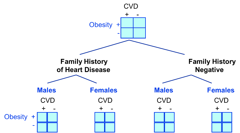
In looking at the relationship between exercise and heart disease we were also concerned about confounding by other factors, such as gender and the presence of a family history of heart disease. We could also stratify by these factors to see if they were confounders and to adjust for them.

Limitations of Stratified Analysis

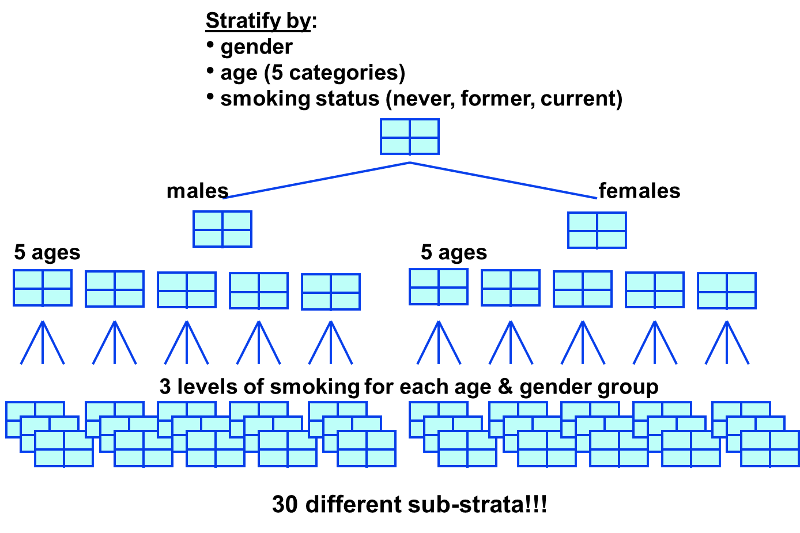
A stratified analysis is easy to do and gives you a fairly good picture of what's going on. However, a major disadvantage to stratification is its inability to control simultaneously for multiple confounding variables. For example, you might decide to control for gender, 3 levels of smoking exposure, 4 levels of age, and 4 levels of BMI. This would require 96 separate strata to control for all of these variables simultaneously, and as you increase the number of strata, you keep whittling away at the number of people in each stratum, so sample size becomes a major problem, since many of the strata will contain few or no people.

Summary of Control of Confounding

Effect Measure Modification

The term effect modification is applied to situations in which the magnitude of the effect of an exposure of interest differs depending on the level of a third variable. Reye's syndrome is a rare, but severe condition characterized by the sudden development of brain damage and liver dysfunction after a viral illness. The syndrome is most commonly seen in children between the ages of 4-14 who have been treated with aspirin while recovering from a viral illness, most commonly chickenpox or influenza. Fortunately, Reye's syndrome has become very uncommon since aspirin is no longer recommended for routine use in children. While Reye's syndrome can occur in adults, it is distinctly more common in children. Thus, the effect of aspirin treatment for a viral illness is very clearly modified by age.

In this situation, computing an overall estimate of association is misleading. One common way of dealing with effect modification is examine the association separately for each level of the third variable. For example, if one were to calculate the odds ratio for the association between aspirin treatment during a viral infection and development of Reye's syndrome, the odds ratio would be substantially greater in children than in adults. As another example, suppose a clinical trial is conducted and the drug is shown to result in a statistically significant reduction in total cholesterol. However, suppose that with closer scrutiny of the data, the investigators find that the drug is only effective in subjects with a specific genetic marker and that there is no effect in persons who do not possess the marker. The effect of the treatment is different depending on the presence or absence of the genetic marker. This is an example of effect modification or "statistical interaction".

Effect Modification with a Continuous Outcome

Evaluation of a Drug to Increase HDL Cholesterol

Consider the following clinical trial conducted to evaluate the efficacy of a new drug to increase HDL cholesterol (the "good" cholesterol). One hundred patients are enrolled in the trial and randomized to receive either the new drug or a placebo. Background characteristics (e.g., age, sex, educational level, income) and clinical characteristics (e.g., height, weight, blood pressure, total and HDL cholesterol levels) are measured at baseline, and they are found to be comparable in the two comparison groups. Subjects are instructed to take the assigned medication for 8 weeks, at which time their HDL cholesterol is measured again. The results are shown in the table below.    

On average, the mean HDL levels are 0.95 units higher in patients treated with the new medication. A two sample test to compare mean HDL levels between treatments has a test statistic of Z = -1.13 which is not statistically significant at α=0.05.  

Based on their preliminary studies, the investigators had expected a statistically significant increase in HDL cholesterol in the group treated with the new drug, and they wondered whether another variable might be masking the effect of the treatment. Other studies had, if fact, suggested that the effectiveness of a similar drug was différèrent in men and women. In this study, there are 19 men and 81 women. The table below shows the number and percent of men assigned to each treatment. 

There is no meaningful difference in the proportions of men assigned to receive the new drug or the placebo, so sex cannot be a confounder here, since it does not differed in the treatment groups. However, when the data are stratified by sex, they find the following:

On average, the mean HDL levels are very similar in treated and untreated women, but the mean HDL levels are 6.19 units higher in men treated with the new drug. This is an example of effect modification by sex, i.e., the effect of the drug on HDL cholesterol is different for men and women. In this case there is no apparent effect in women, but there appears to be a moderately large effect in men. (Note, however, that the comparison in men is based on a very small sample size, so this difference should be interpreted cautiously, since it could be the result of random error or confounding.

When there is effect modification, analysis of the pooled data can be misleading. In this example, the pooled data (men and women combined), shows no effect of treatment. Because there is effect modification by sex, it is important to look at the differences in HDL levels among men and women, considered separately. In stratified analyses, however, investigators must be careful to ensure that the sample size is adequate to provide a meaningful analysis.  

Effect Modification with a Dichotomous Outcome

Consider the following hypothetical study comparing hospitalization after a motor vehicle collision for male and female drivers.

Crude Data:

Crude risk ratio=1.44

Age-Stratified:

Age ‹40

Stratum-specific risk ratio=1.80

Age ≥40

Stratum-specific risk ratio=0.93

In this case, the crude analysis suggests an association between male gender and frequency of hospitalization for motor vehicle collisions. However, if we stratify this by age, we see a strong association with male gender in subjects <40 years old, but no association in subjects 50+. Perhaps males <40 years old driver more recklessly than their female counterparts, but after age 40 driving aggression becomes similar in males and females.

Another good example of effect modification is seen with skin cancers. It is well established that excessive exposure to UV irradiation increases one's risk of skin cancer. However, the risk of UV-induced skin cancer is 1,000 times greater in people with xeroderma pigmentosum. This is a rate hereditary defect (autosomal recessive) in the enzyme system that repairs UV-induced damage to DNA. It is characterized by photosensitivity, pigmentary changes, premature skin aging, and greatly increased susceptibility to malignant tumor development.

If effect modification is present, it is NOT appropriate to use Mantel-Haenszel methods to combine the stratum-specific measures of association into a single pooled measurement. Effect modification is a biological phenomenon that should be described, so the stratum-specific estimates should be reported separately. In contrast, confounding is a distortion of the true association caused by an imbalance of some other risk factor.

• If there is only confounding: The stratum-specific measures of association will be similar to one another, but they will be different from the overall crude estimate by 10% or more. In this situation, one can use Mantel-Haenszel methods to calculate a pooled estimate (RR or OR) and p-value.
• If there is neither confounding nor effect modification: The crude estimate of association and the stratum-specific estimates will be similar. They don't have to be identical, just similar.
• If there is only effect modification: The stratum-specific estimates will differ from one another significantly. Whether they are "significantly different" can be tested by using a chi-square test of homogeneity, as described in the Aschengrau & Seage textbook.
• If there is both effect modification and confounding: Here, you need to consider two possibilities:

1) If the stratum-specific estimates differ from one another, and they are both less than the crude estimate or if they are both greater than the crude estimate, then there is both confounding and effect modification.

2) If the stratum-specific estimates differ from one another, and the crude estimate is between the two stratum-specific estimates, then you need to pool the stratum-specific estimates (with a Mantel-Haenszel equation) to determine whether the pooled estimate is more than 10% different from the crude estimate.

Note that in this situation you are only pooling the stratum-specific estimates in order to make a decision about whether confounding is present; you should not report the pooled estimate as an "adjusted" measure of association if there is effect modification

Statistical Interaction versus Biological Interaction

While the discussion above provides a standard description of effect modification, but on closer scrutiny the concept of effect modification is more complicated than this. Consider the figure below (adapted from KJ Rothman: Epidemiology - An Introduction, Oxford University Press, 2002.) We see two scenarios in which incidence rates in exposed and unexposed individuals are assessed at different ages. Rate ratio and rate difference are both measures of effect, but depending on which we use, our conclusions about effect modification differ.

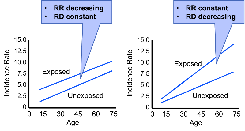
In the first scenario the rate difference remains constant across the spectrum of age, suggesting no effective modification. However, the rate ratio decreases with increasing age (RR=3 at age 15; RR=1.5 at age 75). In the second scenario the rate ratio remains relatively constant, but the rate difference increases with age. Our conclusion regarding whether or not there is effect modification will depend on which measure of effect we use.

Consider also the hypothetical data on the risk of lung cancer in smokers and non-smokers, both with and without exposure to asbestos (also adapted from Rothman).

Table - Hypothetical 1-Year Risk of Lung Cancer per 100,000

First consider the effect of asbestos on the risk associated with smoking. The risk ratio is 5 both with and without asbestos exposure, suggesting no effect modification. However, the risk difference 4 per 100,000 without asbestosis and 40 per 100,000 with asbestosis exposure. This effect measure is clearly modified by asbestos. We can also look at the effect of smoking on the risk associated with asbestos. The risk ratio for asbestos exposure compared to no asbestos exposure is 10 in both smokers and non-smokers, suggesting an absence of effect modification. However, the risk difference is 45 per 100,000 in the presence of smoking, but only 9 per 100,000 in the absence of smoking. Thus, the risk ratios suggest no effect modification, but the risk differences suggest substantial effect modification.

Rothman argues that this ambiguity regarding effect measure modification and statistical interaction makes it important to make a distinction between statistical interaction (which is ambigous) and biological interaction (which is not ambiguous; it is either present or absent.) Biological interaction between two causes occurs if the effect of one is dependent on the presence of the other. For example, exposure to the measles virus is a component cause of developing measles, but it is dependent on another factor, i.e., the immune status of the exposed individual. Someone who is immune because of vaccination or having already had measles will not experience any effect from exposure to the measles virus. A discussion of the methods for measuring biological interaction is beyond the scope of this module. Those who are interested should refer to the discussion in Rothman's excellent text.

The director of the surgical trauma service at Boston Medical Center suspected that elderly drivers (age 70+) had inordinately poor outcomes compared to younger drivers after being in a motor vehicle collision (MVC). His research hypothesis was tested using data from the Boston Medical Center Trauma registry and data from the National Trauma Data Bank.

1. Are there any factors that might confound the association between being al elderly driver and the risk of death after a motor vehicle collision? If so, what factors would you consider? How would you deal with these potential confounders?
2. The figure below summarizes some of the data obtained from the Boston Medical Center Trauma registry. The upper contingency table shows deaths among the 74 elderly drivers hospitalized after an MVC and the 960 younger drivers who had been hospitalized after an MVC. The lower two tables summarize the findings after stratifying based on whether the drivers had the benefit of safety devices (seat belt buckled and/or air bag in the vehicle. Do these findings suggest the presence of effect modification? Why or why not?

Crude Analysis:

Stratified by Use of a Safety Restraint:

Unrestrained (no seatbelt or air bag):

Restrained with Seatbelt, Air Bag, or Both

Try to answer these questions on your own. Then proceed to the next page to see the answers.

Answer to Final Questions Regarding Death Rates in Elderly Drivers

1. Are there any factors that might confound the association between being al elderly driver and the risk of death after a motor vehicle collision? If so, what factors would you consider? How would you deal with these potential confounders?
2. The figure below summarizes some of the data obtained from the Boston Medical Center Trauma registry. The upper contingency table shows deaths among the 74 elderly drivers hospitalized after an MVC and the 960 younger drivers who had been hospitalized after an MVC. The lower two tables summarize the findings after stratifying based on whether the drivers had the benefit of safety devices (seat belt buckled and/or air bag in the vehicle. Do these findings suggest the presence of effect modification? Why or why not?

Crude Analysis:

Crude risk ratio = 6.75

Stratified by Use of a Safety Restraint:

Unrestrained (no seatbelt or air bag):

Stratum-specific risk ratio= 9.54

Restrained with Seatbelt, Air Bag, or Both

Stratum-specific risk ratio= 4.90

Answers:

1. One can think of a number potential confounding factors such as speed of the two vehicles, type of vehicle (e.g., a small light car versus a sturdy vehicle with good protection, site of impact (driver's side versus passenger side), severity of injuries, general health of the the driver prior to the accident, etc. One could explore confounding by these factors by first performing a series of stratified analyses. One might then use multiple logistic regression to simultaneously adjust for several confounding factors.
2. The risk of death was substantially greater in elderly drivers regardless or restratint use. However, unrestrained elderly drivers had almost a ten-fold increase in death rate compared to younger drivers, whereas restrained elderly drivers had a five fold increase in death rates compared to younger drivers. Therefore the effect of age on risk of death after a car crash was different depending on wether restraints were in use. There is good evidence for effect modification here because the stratum-specific measures of association are substantially different.

.