


Tools for Evaluating Linear Relationships Between Continuous Variables
When looking for a potential association between two measurement variables, we can begin by creating a scatter plot to determine whether there is a reasonably linear relationship between them. The possible values of the exposure variable (i.e., predictor or independent variable) are shown on the horizontal axis (the X-axis), and possible values of the outcome (the dependent variable) are shown on the vertical axis (the Y-axis).
In the hypothetical example below an individual's accumulated savings over time are plotted as a function of time in weeks. There is some scatter to the data points, but there is the general sense that the overall trend is a linear increase over time. We might ask how closely the accumulation of savings correlates with time or ask about the average savings per week, and we might also ask about the probability that the apparent relationship is just the result of random error (chance).
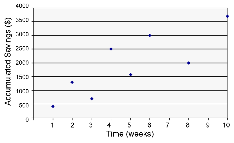
In fact, we can answer these questions by using correlation analysis and simple linear regression analysis, as illustrated in the graph below.
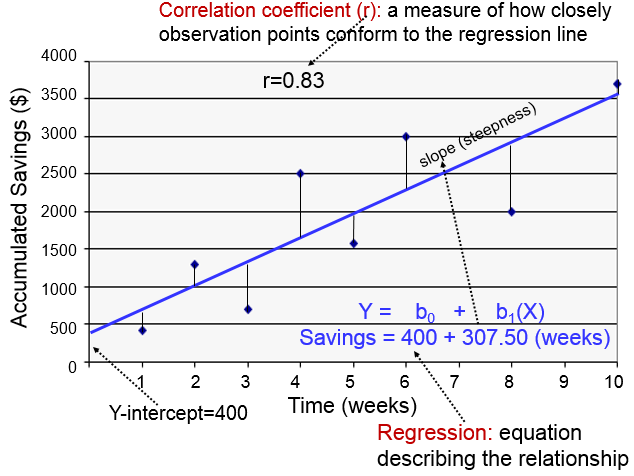
The regression line is determined from a mathematic model that minimizes the distance between the observation points and the line. How closely the individual observation points conform to the regression line is measured by the correlation coefficient ("r"). The steepness of the line is the slope, which is a measure of how many units the Y-variable changes for each increment in the X-variable; in this case the slope provides an estimate of the average weekly increase in savings. Finally, the Y-intercept is the value of Y when the X value is 0; one can think of this as a starting or basal value, but it is not always relevant. In this case, the Y-intercept is $400 suggesting that this individual had that much in savings at the beginning, but this may not be the case. She may have had nothing, but saved a little less than $500 after one week.
Notice also that with this kind of analysis the relationship between two measurement variables can be summarized with a simple linear regression equation, the general form of which is:

where b0 is the value of the Y-intercept and b1 is the slope or coefficient. From this model one can make predictions about accumulated savings at a particular point in time by specifying the time (X) that has elapsed. In this example, the equation describing the regression is:
SAVINGS=400 + 307.50 (weeks)
If I wanted to predict how much money had been saved after 5 weeks, I could substitute X=5 for the number of weeks as follows: SAVINGS = 400 + 307.50(5)= $1.937.50. Note that this is a bit more than the actual savings at that time.