Module 7 - Comparing Continuous Outcomes
When trying to accurately estimate the strength of association between an exposure and an outcome, there are several sources of error that must be considered:
Random errors are errors that arises from sampling. Just by chance the estimates from samples may not accurately reflect an association in the population from which the samples are drawn. In this module we will discuss how to evaluate random error when dealing with continuous outcomes. The statistical significance of these comparisons is often evaluated by computing a confidence interval or a p-value.
We will consider the relevance of p-values for population health science research, and we will also consider the limitations of using p-values to determine "statistical significance" when comparing groups. We will specifically address the common use of t-tests for evaluating associations between two continuous variables, for example, to determine whether people who are obese have a greater risk of having high blood pressure.
After successfully completing this section, the student will be able to:
Our general strategy is to specify a null and alternative hypothesis and then select and calculate the appropriate test statistic, which we will use to determine the p-value, i.e., the probability of finding differences this great or greater due to sampling error (chance). If the p-value is very small, it indicates a low probability of observing these difference as a result of sampling error, i.e., the null hypothesis is probably not true, so we will reject the null hypothesis and accept the alternative.
For continuous outcomes, there are three fundamental comparisons to make:
where
(There is also a procedure called analysis of variance (ANOVA) for comparing the means among more than two groups, but we will not address ANOVA in this course.)
Notice that all three of these tests generate a test statistic that takes into account:
A test statistic enables us to determine a p-value, which is the probability (ranging from 0 to 1) of observing sample data as extreme (different) or more extreme if the null hypothesis were true. The smaller the p-value, the more incompatible the data are with the null hypothesis.
A p-value ≤ 0.05 is an arbitrary but commonly used criterion for determining whether an observed difference is "statistically significant" or not. While it does not take into account the possible effects of bias or confounding, a p-value of ≤ 0.05 suggests that there is a 5% probability or less that the observed differences were the result of sampling error (chance). Furthermore, while it does not indicate certainty, it suggests that the null hypothesis is probably not true, so we reject the null hypothesis and accept the alternative hypothesis if the p-value is less than or equal to 0.05. The 0.05 criterion is also called the "alpha level," indicating the probability of incorrectly rejecting the null hypothesis.
A p-value > 0.05 would be interpreted by many as "not statistically significant," meaning that there was not sufficiently strong evidence to reject the null hypothesis and conclude that the groups are different. This does not mean that the groups are the same. If the evidence for a difference is weak (not statistically significant), we fail to reject the null, but we never "accept the null," i.e., we cannot conclude that they are the same – only that there is insufficient evidence to conclude that they are different.
While commonly used, p-values have fallen into some disfavor recently because the 0.05 criterion tends to devolve into a hard and fast rule that distinguishes "significantly different" from "not significantly different."
"A P value of 0.05 does not mean that there is a 95% chance that a given hypothesis is correct. Instead, it signifies that if the null hypothesis is true, and all other assumptions made are valid, there is a 5% chance of obtaining a result at least as extreme as the one observed. And a P value cannot indicate the importance of a finding; for instance, a drug can have a statistically significant effect on patients' blood glucose levels without having a therapeutic effect."
[Monya Baker: Statisticians issue warning over misuse of P values. Nature, March 7,2016]
Consider two studies evaluating the same hypothesis. Both studies find a small difference between the comparison groups, but for one study the p-value =0.06, and the authors conclude that the groups are "not significantly different"; the second study finds p=0.04, and the authors conclude that the groups are significantly different. Which is correct? Perhaps one solution is to simply report the p-value and let the reader come to their own conclusion.
|
Cautions Regarding Interpretation of P-Values
|
Many researchers and practitioners now prefer confidence intervals, because they focus on the estimated effect size and how precise the estimate is rather than "Is there an effect?"
Also note that the meaning of "significant" depends on the audience. To scientists it mean "statistically significant," i.e., that p ≤ 0.05, but to a lay audience significant means "important."
Many public health researchers and practitioners prefer confidence intervals, since p-values give less information and are often interpreted inappropriately. When reporting results one should provide all three of these.
Investigators wanted to determine whether children who were born very prematurely have poorer cognitive ability than children born at full term. To investigate they enrolled 100 children who had been born prematurely and measured their IQ in order to compare the sample mean to a normative IQ of 100. In essence, the normative IQ is a historical or external (μ0). In the sample of 100 children who had been born prematurely the data for IQ were as follows: X̄ = 95.8, SD = 17.5" . The investigators wish to use a one-tailed test of significance.
A research hypothesis that states that two groups differ without specifying direction, i.e., which is greater, is a two-tailed hypothesis. In contrast, a research hypothesis that specifies direction, e.g., that the mean in a sample group will be less than the mean in a historic comparison group is a one-tailed hypothesis. Similarly, a hypothesis that a mean in a sample group will be greater than the mean in a historic comparison group is also a one-tailed hypothesis.
Suppose we conduct a test of significance to compare two groups (call them A and B) using large samples. The test statistic could be either a t score or a Z score, depending on the test we choose, but if the sample is very large the t or Z scores will be similar. Suppose also that we have specified an "alpha" level of 0.05, i.e., an error rate of 5% for concluding that the groups differ when they really don't. In other words, we will use p≤0.05 as the criterion for statistical significance.
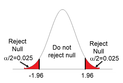
Two-tailed test: The first figure below shows that with a two-tailed test in which we acknowledge that one group's mean could be either above or below the other, the alpha error rate has to be split into the upper and lower tails, i.e., with half of our alpha (0.025) in each tail. Therefore, we need to achieve a test statistic that is either less than -1.96 or greater than +1.96.
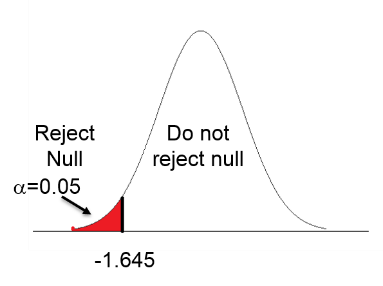
One-tailed test (lower tail): In the middle figure the hypothesis is that group A has a mean less than group B, perhaps because it is unreasonable to think the A would be greater than B. If so, all of the 5% alpha is in the lower tail, and we only need to achieve a test statistic less than 1.645 to achieve "statistical significance."
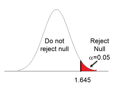
One-tailed test (upper tail): The third image shows a one-tailed test in which the hypothesis is that group A has a mean value greater than that of group B, so all of the alpha is in the upper tail, meaning that we need a test statistic greater than +1.645 to achieve statistical significance.
Clearly, the two-tailed test is more conservative because, regardless of direction, the test statistic has to be more than 1.96 units away from the null. The vast majority of tests that are reported are two-tailed tests. However, there are occasionally situations in which a one-tailed test hypothesis can be justified.
A one-tailed test could be justified in the study examining whether children who had been born very prematurely have lower IQ scores than children who had a normal, full term gestation, since there is no reason to believe that those born prematurely would have higher IQs.
First, we set up the hypotheses:
Null hypothesis: H0: μprem = 100 (i.e., that there is no difference or association)
Children born prematurely have mean IQs that are not different from those of the general population (μ0=100)
Alternative hypothesis (research hypothesis: H0:μprem < 100)
Children born prematurely have lower mean IQ than the general population (μ<100).
The t statistic= -2.4. We can look up the corresponding p-value with df=99, or we can use R to compute the probability.
> pt(-2.4,99)
[1] 0.009132283
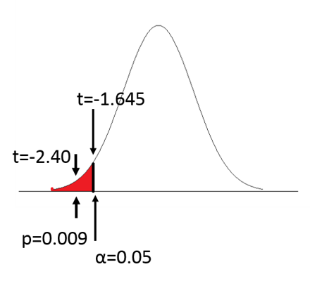
Since p=0.009, we reject the null hypothesis and accept the alternative. We conclude that children born prematurely have lower mean IQ scores than children in the general population who had a full term gestation.
What if we had performed a two-tailed test of hypothesis on the same data?
The null hypothesis would be the same, but the alternative hypothesis would be:
Alternative hypothesis(research hypothesis: HA: μprem≠100
Children born prematurely have IQ scores that are different (either lower or higher) from children from the general population who had full term gestation.
The calculation of the t statistic would also be the same, but the p-value will be different.
> 2*pt(-2.4,99)
[1] 0.01826457
The probability (area) either lower than -2.40 or greater than +2.40 = 0.009+0.009 =0.018, i.e., we have a probability of 0.009 in both the lower and upper tail. We still conclude that children born prematurely have a significantly lower mean IQ than the general population (mean=95.8, s=17.5, p=0.018).
[When performing two-tailed tests, direction is not specified in the hypothesis, but one should report the direction in any report, publication, or presentation, e.g., "Children who had been born prematurely had lower mean IQ scores than in the general population."]
|
Student's t-test
The t-statistic was developed and published in 1908 by William Gosset, a chemist/statistician working for the Guinness brewery in Dublin. Guinness employees were not allowed to publish under their own name, so Gosset published under the pseudonym "Student". |
In the example for IQ tests above we were given the mean IQ and standard deviation for the children who had been born prematurely. However, suppose we were given an Excel spreadsheet with the raw data listed in a column for "iq"?
In Excel we could save this data as a .CSV file using the "Save as" function. We could then import the data in the .CSV file into R and analyze the data as follows:
[Note that R defaults to performing the more conservative two-tailed test unless a one-tailed test is specified as we will describe below.]
> t.test(iq,mu=100)
One Sample t-test
data: iq t = -2.3801, df=99, p-value = 0.01922
alternative hypothesis: true mean is not equal to 100
95 percent confidence interval:
92.35365 99.30635
Sample estimates
mean of x
95.83
In order to perform a one-tailed test, you need to specify the alternative hypothesis. For example:
> t.test(iq,mu=100, alternative="less")
or
> t.test(iq,mu=100, alternative="greater")
Hypothesis tests do not provide certainty, only an indication of the strength of the evidence. In essence, "alpha" =0.05 is an error rate of 5% when rejecting the null hypothesis and accepting the alternative hypothesis. This is referred to as a Type I error. In contrast, a Type II error occurs when there really is a difference, but we fail to reject the null hypothesis.
| Truth | H0 Not Rejected (Insufficient Evidence of a Difference) |
H0 Rejected (Difference) |
| H0 true | Correct | Type I error |
| H0 false | Type II error | Correct |
Type I Error: Concluding that there is a difference when there isn't
Type II Error: Concluding no difference when there really is one.
Suppose investigators want to assess the effectiveness of a new drug in lowering cholesterol, and they want to conduct a small clinical trial in which patients were randomized to receive the new drug or placebo, and total cholesterol was measured after six weeks on the assigned treatment. The table below shows the results.
| Sample Size (n) | Mean Cholesterol (6 wk) | SD | |
| New drug | 15 | 195.9 | 28.7 |
| Placebo | 15 | 217.4 | 30.3 |
Is there sufficiently strong evidence of a difference in mean cholesterol for patients on the new drug compared to patients receiving the placebo?
Note that SD is used to characterize individual variability within each group, although we will use SE when conducting a hypothesis test to compare the means.
H0: μ1 = μ2
H1:μ1≠ μ2
Since we are comparing the means in two independent groups (i.e., different patients in the two treatment groups), we will use the two independent sample t-test (aka, unpaired t-test) shown below. "Sp" is the pooled standard deviation for the two groups.
where
Use of this test assumes that the variance for the two groups are more or less equal. Recall that variance = the square of the standard deviation, and note that s12 and s22 are the variances for the two samples, and they are included in the calculation of Sp. We can test the assumption of equal variance by computing the ratio of the two variances, and if the ratio is in the range of 0.5 to 2.0, then the assumption is adequately met. If this is not the case, a different equation must be used (the Welch t-test), but if we are using R, there is a simple way to make this adjustment, as you will see.
In the example we are currently using the ratio of the variances is
Ratio = 28.72 / 30.32 = 0.90
so the assumption is met.
Next, we need to compute the pooled standard deviation.
So, Sp=29.5 will be plugged into the equation for the test statistic as shown in the next step.
df = n1 + n2 - 2 = 28
We can use R to compute the two-tailed p-value:
2*pt(-2.92,28)
[1] 0.006840069
The p-value is 0.007, so there is sufficient evidence to reject the null hypothesis.
Conclusion:
Mean cholesterol is statistically significantly lower in patients on treatment as compared to placebo: 195.9 ± SD: 28.7 vs. 217.4 ± SD: 30.3, p=0.007).
In order to test whether the mean age of people who drank alcohol differed from that of non-drinkers, the following code was used in R:
> t.test(Age~Drink,var.equal=TRUE)
Two Sample t-test
data: Age by Drink
t= 2.4983, df=2189, p-value = 0.01255
alternative hypothesis: true differences in means is not equal to 0
95 percent confidence interval:
0.140054 1.1624532
sample estimates:
mean in group No mean in group Yes
25.54535 24.89410
In the example above, the two means are 25.4535 and 24.89410. The difference in means = 0.65125. Notice that R gives the 95% confidence interval for the difference in the means for the two groups (0.140054, 1.1624532). The null for the difference in means is 0, and if the 95% confidence interval for the difference in means does not contain the null value, then the p-value must be < 0.05 if we are using a two-tailed test. Therefore, the observation that the 95% confidence interval does not contain the null value of 0 is consistent with the p-value= 0.01255.
Example: Long-term Developmental Outcomes in Infants with Iron Deficiency
Lozoff and colleagues compared developmental outcomes in children who had been anemic in infancy to those in children who had not been anemic. Physical and mental development were compared between children with versus without a history of iron deficiency anemia. Physical development was assessed by computing the mean gross motor composite score. Mental development was assessed by measuring mean IQ scores in each group. Statistical significance was evaluated using the two independent sample t-test. Some results are shown in the table below.
| Gross Motor | Verbal IQ | |
| Children w iron deficiency (n=30) Children w/o deficiency (n=133) |
52.2 ± 13.0 58.8 ± 12.5 |
101.4 ± 13.2 102.9 ± 12.4 |
| Difference in means 95% CI for difference in means |
-6.6 (-11.6, -1.6) |
-1.5 (-6.5, 3.5) |
| p-value | p=0.010 | p=0.556 |
The difference in means for gross motor scores was -6.5 with a 95% confidence interval from -11.6 to -1.6. The null value of 0 difference is not included inside the confidence interval, indicating that the p-value must be <0.05, and as you can see it is 0.01. However, for verbal IQ the mean difference was -1.5 with a 95% confidence interval from -6.5 to 3.5. This confidence interval does include the null value of 0, indicating that the p-value must be >0.05, and as you can see the p-value for verbal IQ is 0.556 indicating that the difference is not statistically significant.
If the sample variances do not meet the equal variance assumption, R can easily compute this using the Welch t-test by simply changing "var.equal=TRUE" to "var.equal=FALSE" as shown below.
> t.test(Age~Drink,var.equal=FALSE)
The third application of a t-test that we will consider is for two dependent (paired or matched) samples. This can be applied in either of two types of comparisons.
Example 1: Does Intervention Increase HIV Knowledge?
Early in the HIV epidemic, there was poor knowledge of HIV transmission risks among health care staff. A short training was developed to improve knowledge and attitudes around HIV disease. Was the training effective in improving knowledge?
Table - Mean ( ± SD) knowledge scores, pre- and post-intervention, n=15
| Pre-Intervention | Post-Intervention | Change |
| 18.3 ± 3.8 | 21.9 ± 4.4 | 3.53 ± 3.93 |
The raw data for this comparison is shown in the next table.
|
Subject |
Kscore1 | Kscore2 | difference |
|
1 |
17 | 22 | 5 |
|
2 |
17 | 21 | 4 |
|
3 |
15 | 21 | 6 |
|
4 |
19 | 26 | 7 |
|
5 |
18 | 20 | 2 |
|
6 |
14 | 14 | 0 |
|
7 |
27 | 31 | 4 |
|
8 |
20 | 18 | -2 |
|
9 |
12 | 22 | 10 |
|
10 |
21 | 20 | -1 |
|
11 |
20 | 27 | 7 |
|
12 |
24 | 23 | -1 |
|
13 |
17 | 15 | -2 |
|
14 |
17 | 24 | 7 |
|
15 |
17 | 24 | 7 |
| mean difference = | 3.533333 | ||
| sddiff= | 3.925497 | ||
| p-value= |
0.003634 |
The strategy is to calculate the pre-/post- difference in knowledge score for each person and determine whether the mean difference=0.
First, establish the null and alternative hypotheses.
Then compute the test statistic for paired or matched samples
For the example above we can compute the p-value using R. First, we compute the means.
> mean(Kscore1)
[1] 18.33333
> mean(Kscore2)
[1] 21.86667
Then we perform the t-test for two dependent samples.
> t.test(Kscore2,Kscore1,paired=TRUE)
Paired t-test
data: Kscore2 and Kscore1 t = 3.4861, df = 14, p-value = 0.003634
alternative hypothesis: true difference in means is not equal to 0
95 percent confidence interval:
1.359466 5.707201
sample estimates:
mean of the differences
3.533333
The null hypothesis is that the mean change in knowledge scores from before to after is 0. However, the analyis shows that the mean difference is 3.53 with a 95% confidence interval that ranges from 1.36 to 5.7. Since the confidence interval does not include the null value of 0, the p-value must be < 0.05, and in fact it is 0.003634.
The report by Lozoff et al. found the following results:
| Gross Motor | Verbal IQ | |
| Children w iron deficiency (n=30) Children w/o deficiency (n=133) |
52.2 ± 13.0 58.8 ± 12.5 |
101.4 ± 13.2 102.9 ± 12.4 |
| Difference in means 95% CI for difference in means |
-6.6 (-11.6, -1.6) |
-1.5 (-6.5, 3.5) |
| p-value | p=0.010 | p=0.556 |
One good way of reporting on this would be:
Children with a history of anemia had statistically significant lower gross motor function scores than the comparison children who did not have anemia (difference in means: -6.6 points; 95% confidence interval: -11.6,-1.6; p=0.016). There was no statistically significant difference verbal IQ scores (difference in means: -1.5 points; 95% confidence interval -6.5, 3.5; p=0.556).