
PH717 Module 2 - Exposure Assessment
In order to prevent or mitigate adverse health effects, we must identify potentially harmful exposures, identify their sources, identify persons who are exposed, and then quantify their extent of exposure and assess their risk of adverse health effects. We can then use this information to reduce harmful exposures, thereby reducing risk and reducing adverse health effects.
The goal of human exposure assessment is to estimate and quantify human contact and entry into the body of potentially harmful agents. This includes:
Essential Questions:
After completing this section, you will be able to:
Levin et al, 2004. Physical health status of World Trade Center Rescue and Recovery Workers and Volunteers – New York City, July 2002-August 2004. Mortality and Morbidity Weekly Report, Centers for Disease Control and Prevention
Exposure may be defined as contact of an organism with any measurable chemical, physical, or biological agent that affects health. This can include variables or factors across a broad spectrum from the molecular level all the way up to the social and political environment. Certainly, there are many specific chemical, biological, or physical agents that can be transmitted through environmental media (air, water, food, soil). However, exposures can also be thought of more broadly to include the social contacts, cultural practices, regulations, policies, and laws that people live with every day. These are also potentially important determinants of health. This broad array of potentially relevant exposures is encompassed by the socio-ecologic model as illustrated in the graphic below.

For example, areas with higher taxes on alcohol have lower alcohol consumption rates, and several studies have found that citywide bans on public smoking reduce the incidence of acute myocardial infarction.
Measurable means we can measure, estimate, or classify the exposure.
Many exposures can be measured on a continuous scale, such as measuring PM2.5 in air (fine particulate air pollution measuring less than 2.5 microns in diameter). Many other exposures cannot be measured on a continuous scale, but they can be categorized using variables that are:
The conceptual model for understanding the link between environmental exposures and adverse health outcomes is shown below. Note that exposure assessment embraces the first five steps from identification of the source to estimation of the absorbed dose.
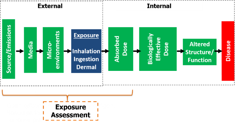
The goal of human exposure assessment is to identify and quantify exposures to chemical, physical, and biological agents that may have adverse health effects. This includes:
Armed with this information, it becomes feasible to formulate strategies to prevent or mitigate adverse health effects.
Several aspects of exposure assessment merit particular emphasis:
The duration of exposure may have an important impact on the likelihood of adverse consequences.
There are three categories of duration of exposures:
By acute exposures we mean short-term exposures to an agent (or experience) which may or may not be repeated
Examples:
These are exposures that are present for long periods of time; possibly constant; possibly life-long.
Examples:
Time-varying exposures are those that vary across the life course of an individual, such as beginning to smoke and gradually increasing the amount, then quitting. Other time-varying exposures might include:
Examples:
Estimating the overall dose of exposure is complicated, since it can be influenced by:
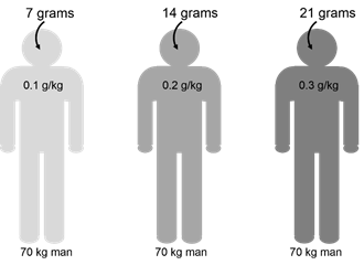
For example, rough estimates might be calculated as follows:
Body size also matters. At a given body weight, the internalized concentration will increase as the amount of contaminant ingested increases.
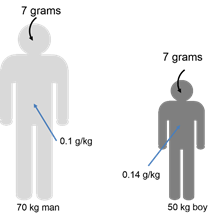
Conversely, if the same amount of a contaminant is ingested by two people of different body weights, the smaller person will have a higher concentration of the contaminant.

In the 1950s and 1960s pregnant women with tenuous pregnancies were often prescribed a drug called diethylstilbestrol (DES). Years later it was found that the in utero exposure to DES caused cancer of the vagina in exposed offspring 15 to 22 years later. This is an example of both critical window (exposure in utero) and long latency.
A more recent example of a critical window is infection of pregnant women with Zika virus, causing microcephaly (smaller than normal head and underdeveloped brain) in their babies.
The illustration below shows a time line of fetal development of each of the major organ systems during pregnancy. Blue bars show critical windows for development of major congenital defects in each organ system, and turquoise bars show critical windows for minor congenital defects.
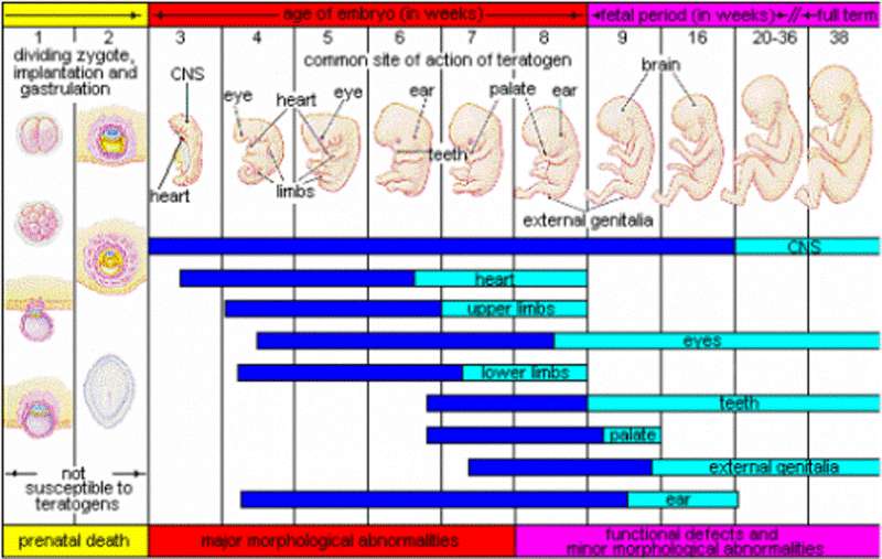
Source: US Environmental Protection Agency (EPA)
https://www.epa.gov/sites/production/files/2014-04/childrens_health_1.gif
The dose of an environmental exposure depends on the amount of contaminant in the media (air, food, etc.), and the level of human contact with that media, i.e., how much was inhaled, ingested, or adsorbed or absorbed by the skin. These are components of the conceptual model used by environmental health scientists.
|
Four Basic Methods for Obtaining Data on Exposure: 1. Self-reporting 2. Monitoring the environment around an individual or in a geographic area 3. Measuring biomarkers: Measure markers of exposure in the individual's body 4. Modeling techniques
|
Self-reported information on exposures can be collected using questionnaires and interviews asking about behaviors, ambient environment, purchasing, diet (e.g., a food frequency questionnaire), medical history, etc. Self-reporting is most useful for personal habits and medications used, and some exposures can only be assessed with self-reports (e.g., sexual practices and recreational drug use). Self-reporting has clear limitations in that people may not accurately remember past exposures, or they may have difficulty quantifying them accurately (e.g., "How much did you exercise?").
In addition, environmental exposures to contaminants in air or water cannot be accurately quantified by self-report and often require a formal exposure assessment to estimate human contact with contaminants.
There are many devices that provide a means of monitoring exposures to particulate matter in the air and to volatile organic compounds such as benzene. The Clean Air Act requires the US EPA to set standards for air quality and to monitor air quality throughout the United States.
Monitors are available to be used in several levels.
Air Sampling of Particulate Matter: There are several methods available for actively sampling particulate matter. Size-selective sampling is the collection of one particle size fraction, such as the collection of PM10 or PM2.5, i.e. particles in the air measuring less than 10 microns or less than 2.5 microns..
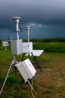
Image source: https://archive.epa.gov/emergency/bpspill/web/html/air-mon.html
Active Sampling of Gases and Vapors: A sampling pump is required to actively sample gases and vapors. One method involves the use of sorbent tubes, which contain collection materials such as activated charcoal, silica gel, tenex, etc.
Passive Sampling of Gases/Vapors: Passive sampling does not require a pump. Passive samplers have been developed for many gaseous pollutants, such as NO2, O3, and volatile organic compounds (VOCs). The sampling rate is controlled by a physical process, such as diffusion through a static air layer or permeation through a membrane.
e.g., in a home or workplace

Measuring exposure in a specific individual using a portable or personal sampling device attached to the individual or placed where the individual spends time.


|
Advantages and Disadvantages of Monitoring Advantages: Community, home, workplace, and personal monitoring is objective, quantitative, and usually continuous. Disadvantages: It is expensive and time consuming, and community biomonitoring may not accurately capture exposure level for every subject. In addition, personal biomonitoring is not feasible for large numbers of people.
|
Biomarkers are biochemical, physiological, and histological changes that can be used to estimate either exposure to chemicals or the effects of exposure to chemicals. Some examples of biomarker samples include blood, urine, hair, and fatty tissue. Because of the invasive nature of biomarker collection, it is often difficult to use them for exposure assessment. Ideally, measurement of a biomarker might provide information about internal dosage of potentially harmful substances.
Non-invasive sampling utilizes breath tests, urine samples, nasal swabs, buccal swabs, sputum, breast milk, semen, hair, nail clippings, or fecal samples.
Invasive sampling refers to blood tests or tissue biopsies.
Biomarkers provide a means of estimating the internal dose of a contaminant that is specific for a single person. Examples of biomarkers include:
|
Advantages and Disadvantages to Biomarkers
Advantages: They are objective, quantitative, and provide an accurate measure of an individual's internal dose. Biomarkers can be collected and monitored across the population to gain insight into trends and subgroups at risk. Disadvantages: They can be expensive, and measurements at a particular point in time may not accurately reflect exposure over a broad period of time.
|
Examples:
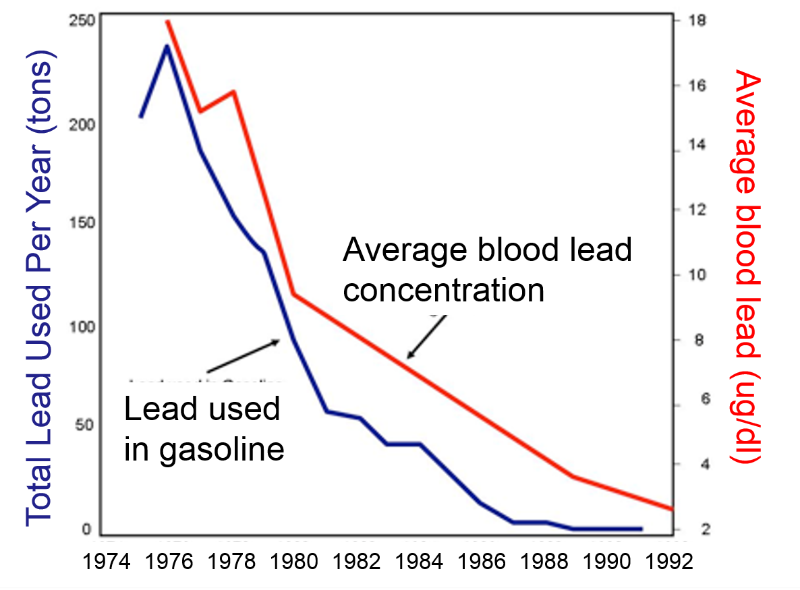
The image below shows that average blood levels of lead in the US population (red line) fell dramatically in parallel with reductions in the amount of lead used as an additive to gasoline (blue line).
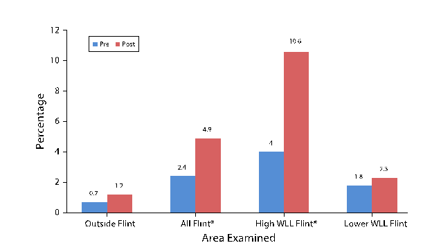
The graph below shows that the percentage of people with high blood levels in Flint, Michigan increased substantially after their water source changed from Lake Huron to the Flint River.
Community, area and personal biomonitoring are all potentially useful in specific circumstances. Personalized assessments of exposure can be particularly useful by providing investigators with individual exposure data. However, personal biomonitoring is expensive and limits the number of people for whom data is available.
Mathematical modeling is a fourth method of obtaining exposure data, and it is attractive because the other methods can be difficult, time-consuming, and expensive. However, modeling doesn't provide real measurements; it provides estimates based on a mathematical model which might be in error or might be based on assumptions that don't apply to many of the individuals.
Types of models that have been employed for exposure assessment include:
For example, the Cape Cod Breast Cancer and Environment Study used geographic information system mapping technology (GIS) to assess exposures to pesticides used in cranberry bogs or in areas sprayed for tree pests and also assessed exposure to drinking water contaminated by wastewater or affected by residential, commercial, or industrial land use. GIS was used to calculate distance from each household to these exposures.
Modeling has been particularly useful for assessing the fate and transport of contaminants, i.e., where they are likely to go.
Fate refers to the chemical and physical degradation and transformation of contaminants and their final destination in the environment. Degradation is the breakdown of contaminants, while transformation refers to an alteration in its structure that may render it more or less harmful. Biodegradation is breakdown by microbes. Degradation or transformation can also occur through chemical or physical processes such as oxidation, hydrolysis, or photolysis. in the environment. Oxidation is breakdown that involves loss of electrons, often as a result of reaction with oxygen. Hydrolysis is the splitting of a molecule through a reaction with water. Photolysis is breakdown caused by absorption of light energy. These processes can be influenced by local conditions such as temperature, presence of water or precipitation, abundance of sunlight, and even the presence of other contaminants. Some chemicals are highly resistant to degradation and transformation and tend to persist or accumulate in the environment, such as DDT and polychlorinated biphenyls (PCBs) .
Transport refers to the movement of contaminants within or between environmental media (water, air, food and soil). Contaminants can be transported for short or long distances. For example:
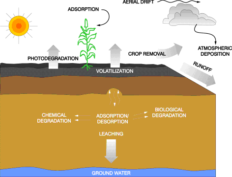
Image source: Source: http://www1.agric.gov.ab.ca/$department/deptdocs.nsf/all/wat3350
Between 1969 and 1986 twenty-one Woburn children were diagnosed with leukemia, and twelve died. Two of the wells supplying drinking water to parts of Woburn were found to be heavily contaminated with trichloroethylene (TCE), an industrial solvent used to dissolve grease and oil. The wells also contained tetrachloroethylene (PCE), also known as perc, Both of these industrial solvents were dumped into the soil by local industry. The solvents were transported by rainwater into the Aberjona River and groundwater aquifers that underlie the city. Eventually the solvents reached wells "G" and "H" that provided drinking water for many Woburn residents. The short video animation below summarizes the movement of the contaminants in groundwater based on the model that was developed.
Animation created by Scott Blair, Ohio State University, Department of Geological Sciences
To learn more about the investigation of the leukemia cluster in Woburn see our online case study at http://sphweb.bumc.bu.edu/otlt/MPH-Modules/woburnleukemia/index.html.
Once a chemical, physical or biological agent reaches us, the exposure route is the way it enters our body. The three major exposure routes to humans are:
Other exposure routes are placental exposure of a fetus, exposure to noise, and eye exposure to ultraviolet (UV) radiation.
The exposure pathway is the physical course an environmental agent takes from its source to those who eventually receive it. For example, agricultural use of pesticides may contaminate crops, the soil, and the air. Some pesticide remains on crops when they are harvested and distributed. Eventually, the food (and the pesticide) are ingested by a human.

The illustration below summarizes a variety of possible exposure pathways.
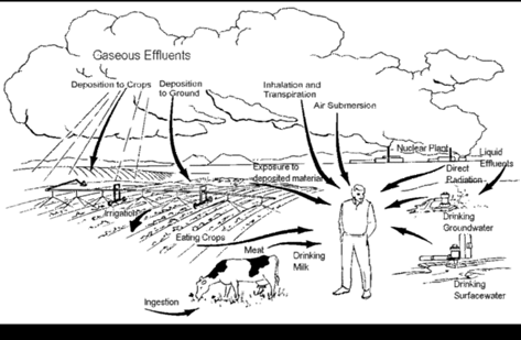
Image source: http://www.atsdr.cdc.gov/hac/pha/PHA.asp?docid=78&pg=2
A key aspect of an exposure pathway investigation is a determination of how people in a community might come into contact with a chemical. In an exposure pathways evaluation, five main elements are considered:
How can we estimate expected health effects from exposure data with limited human-health information?
For many chemicals or compounds we are unsure of the specific health effects, particularly with regard to new products whose health risks are unknown. Toxicology is the study of the adverse effects of chemicals or physical agents on living organisms, including their fate and transport in the body.
ATSDR (Agency for Toxic Substances and Disease Registry) is a US federal agency charged with a variety of functions related to health effects of hazardous substances. These include public health assessments of waste sites, health consultations concerning specific hazardous substances, health surveillance and registries, response to emergency releases of hazardous substances, applied research in support of public health assessments, information development and dissemination, and education and training concerning hazardous substances.
|
Optional Additional Resources
|
How do we know what level dose is harmful?
The relationship between degree of exposure (dose) and magnitude of harmful health effects (toxicity) has generally been addressed by observing how varying doses of an agent influence the frequency or severity of outcomes. Certainly, it would be unethical to purposely expose humans to varying doses of potentially harmful chemicals in order to observe the effects. Consequently, these relationships have been explored most commonly in animals, and the results have been extrapolated to humans.
The Draize test is an acute toxicity test that was introduced in 1944 by FDA toxicologists to test the effects of cosmetics. Measured amounts of the test substance are applied to the eye or the skin of a conscious, restrained rabbit and left there for a fixed amount of time. The substance is then rinsed out, and the animal is observed for up to fourteen days for signs of inflammation (redness, swelling, edema, tenderness) or more severe effects, such as discharge, ulceration, hemorrhage, cloudiness, or blindness. Not surprisingly, the test has been controversial and its use has declined, although it is still recognized by the FDA, since no test has been accepted as an adequate replacement. Anesthetics are now used more commonly, and substances that are known to be toxic are generally not used in Draize tests.
Many other test substances can be tested in animals by injecting it or having them ingest it or inhale it. Since the goal is to relate dosage to toxicity groups of animals would be allocated to receive drugs according to a fixed schedule (e.g., daily) with each group receiving a different dose. The animals would be observed for frequency or severity of clinical outcomes. Acute toxicity tests in the past frequently used death as the definitive outcome. The dose that was lethal in 50% of a group of animals (the LD50) was a standard measurement that enabled one to address relative toxicity.
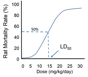
Note that the same concept can be applied to effective doses of drugs. For example, if we were considering the dose of an analgesic that was effective for relieving moderately severe pain from osteoarthritis of the knee, we might consider the effective doses indicated in the table below.
| ED0 |
Dosage that relieves 0% of treated subjects |
| ED10 |
Dosage that relieves 10% of treated subjects |
| ED50 |
Dosage that relieves 50% of treated subjects |
| ED90 |
Dosage that relieves 90% of treated subjects |
It is now more common to observe for non-lethal effects, such as the frequency or severity of tumors, weight loss, behavioral changes, or other abnormalities. Another option is to euthanize animals at fixed intervals of time to examine tissues and body fluids for abnormalities
Still other procedures look for toxic effects of agents using cells grown in culture (in vitro tests rather than in vivo).
The purpose of these tests is to:
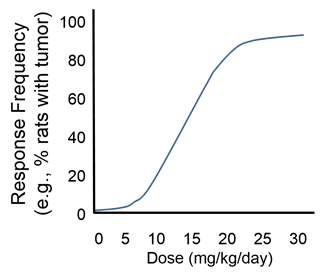
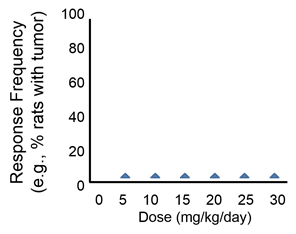
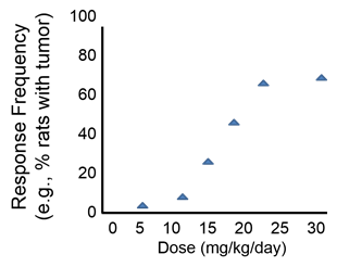
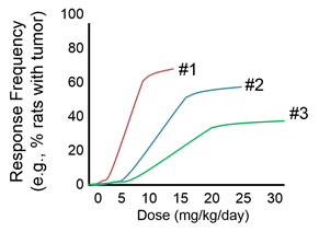
Dose-response curves are frequently sigmoidal, or S-shaped, and for many substances small doses do not appear to be toxic. The point at which toxicity first appears is known as the threshold dose, and the risk of an adverse outcome increases as the dose increases further. This concept is further refined by the terms NOAEL (meaning "no observed adverse effect level") and LOAEL (meaning "lowest observed adverse effect level"). In the example below, a dose of 15 mg/kg/day would represent the threshold dose, which is the LOAEL.
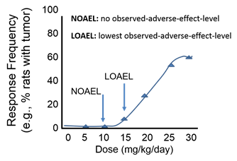
For most non-cancer health outcomes, we assume there is a level dose below which there is no negative health effect. However, carcinogens are generally considered to have no threshold, i.e., no safe dose
|
Advantages and Disadvantages to Animal Studies Advantages
Disadvantages
|
While it would be unethical to allocate humans to receive a potentially harmful substance, it is possible to glean dose-response information from humans in observational studies, i.e., those in which subjects select their own exposures and doses. For example, we have abundant data regarding the effects of alcohol ingestion in humans, as shown in the table below.
|
% Alcohol in Blood |
Observed Effect |
|---|---|
|
0 |
None |
|
0.05-0.1 |
Stimulant; social relaxation |
|
0.1-0.3 |
Increasing lack of coordination |
|
0.3-0.4 |
Loss of consciousness |
|
0.4+ |
Possibly lethal |
Occupational health epidemiology is the study of workplace exposures and associated health effects. Animal studies can provide extremely useful information, but we have already noted some of the limitation, particularly with respect to the tendency to use very high dose for short periods of observation and the issue of extrapolating findings in rodents to humans. However, studies in humans can provide additional information about the toxic effects of chemicals, including chemical exposures in the workplace, exposures in the environment, studies evaluating the safety and efficacy of drugs.
 Question: How would you assess the potential toxicity of the drug shown in the dose-response curve below?
Answer
 Question: How would you interpret the next dose-response curve?
Answer
 Question: How would you assess the dose-response relationships shown in the graph below?
Answer
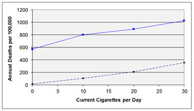
 Question: Consider the information in the graph below, which was constructed based on data from the British Doctors Cohort.
They reported the annual mortality for a variety of disease at four levels of cigarette smoking per day: Never smoked, 1-14/day, 15-24/day, and 25+/day. In order to perform a correlation analysis, we rounded the exposure levels to 0, 10, 20, and 30 respectively, so it is just an approximation, but probably reasonable. The upper curve shows how the incidence of death from cardiovascular disease changes with increased levels of cigarette smoking. The lower curve shows the mortality rate from lung cancer.
How would you asses these dose-response data in humans? Think about how you would interpret this information before you look at the answer.
Answer