PH717 Module 11 - Confounding and Effect Measure Modification
Link to video transcript in a Word file
Most health outcomes are multifactorial, meaning that many factors can influence the risk of developing an outcome, and this complexity often distorts the measurement of association for a relationship we are trying to assess. For example, there are many established risk factors for coronary heart disease (CHD), but suppose we wanted to conduct a prospective cohort study to understand the impact of physical activity on risk of developing CHD. We could enroll a cohort of adults without known CHD and assess their physical activity and perhaps divide the cohort into quintiles based on their physical activity. We could then follow the cohort over time and eventually do an analysis to compare the incidence of CHD among the groups. The problem is that the subjects who exercise the most are probably systematically different from those who exercise the least, and the groups probably differ with respect to other factors that affect the likelihood of CHD developing. People who exercise regularly are likely to be more health conscious, and they are more likely to eat a healthy diet, maintain a healthy weight, get their blood pressure checked regularly, and take vitamins. In addition, they are less likely to smoke and less likely to have diabetes or hypertension. All of these things put them at less risk for CHD, but we want to measure the independent effect of physical activity, i.e., independent of all these other risk factors. When other risk factors that affect the outcome are unequally distributed among our comparison groups, the measure of association will be biased as a result of confounding.
Yet another problem is that the magnitude of association between an exposure and a health outcome might differ depending on the presence of another risk factor. For example, the association between heavy smoking and lung cancer might have a risk ratio of 20 in the general population, but the risk ratio for smoking and lung cancer might be about 60 among shipyard workers who smoke heavily and used to install asbestos in ships as fireproofing. This is a separate phenomenon from confounding called effect measure modification. In essence, it means that the effect of an exposure on an outcome is modified by another factor. In this example, it means that the effect of heavy smoking on risk of lung cancer is greatly magnified among people who also worked with asbestos.
In this module we will take a closer look at confounding and effect measure modification, and you will learn methods of identifying them. Effect measure modification is a biological phenomenon that should be described and reported. In contrast, confounding is just a mathematical distortion, and you will learn ways to prevent confounding and ways to adjust for its distorting effects when it cannot be prevented.
Essential Questions
After completing this section, you will be able to:
Suppose we want to assess the strength of association between physical activity and coronary heart disease (CHD). For simplicity let's assume that we have just two exposure groups:
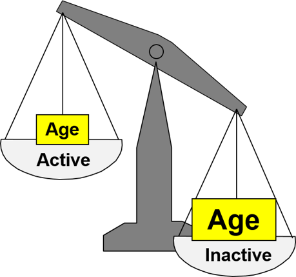
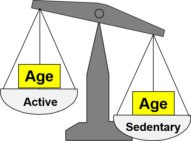
We follow the subjects for ten years and find that the risk ratio for developing CHD in the active group compared to the sedentary group is 0.5, suggesting that those who are physically active have 0.5 times the risk of developing coronary heart disease compared to those who are sedentary. But is this an accurate assessment of the effect of physical activity on risk of CHD?
Older people tend to be less physically active then younger people, and age is clearly a risk factor for coronary heart disease. If the sedentary group is older, how do we separate the impact of physical activity (which we are mainly interested in) from age (which is just another risk factor that confuses things)?
The unequal distribution of age (another risk factor) exaggerates the apparent effect of inactivity. Age differences between active and sedentary people confound the association between activity and CHD. Confounding is the distortion of a measure of association that occurs when other risk factors for the outcome are unevenly distributed between the groups being compared
If the age distribution had been similar in the active and inactive groups, we might have found that the active group had a lower risk of CHD, but the apparent benefit of exercise would have not been as great because age differences were no longer distorting the comparison.
Another exposure can cause confounding if three conditions are met:
1) The additional exposure is an independent risk factor for the outcome under study, i.e., the confounding factor is associated with the outcome. In this example, older age is an independent risk factor for CHD.
2) The distribution of the confounding factor differs among the exposure groups, i.e., it is associated with the exposure. In this example, the sedentary group has a greater proportion of older people.
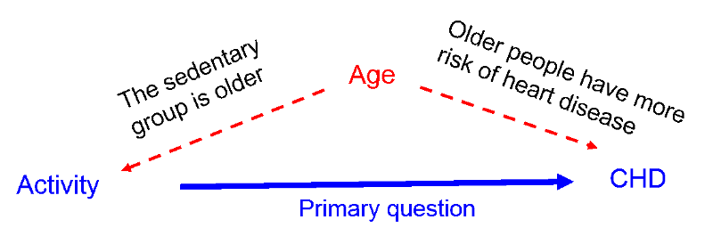
These first two conditions might be depicted by the figure below in which the primary question of interest is the association between activity and CHD, but differences in age distort the measure of association because older people are less active and older people have an inherently greater risk of CHD that is independent of their activity level.
3) A confounding factor cannot be an intermediary factor in the causal pathway between the exposure and the outcome. For example, obesity is a cause of type 2 diabetes, and type 2 diabetes is a cause of coronary heart disease. Given this sequence of events in the causal chain, type 2 diabetes would not be considered a confounding factor for the association between obesity and coronary artery disease, because it is the mechanism by which obesity leads to coronary heart disease.

Later in this module we will discuss methods for adjusting for the distortion caused by confounding. A crude measure of association is one that has not yet been adjusted for confounding factors, while an adjusted measure of association is one that has been adjusted to minimize confounding and provides an estimate that is closer to the true value.
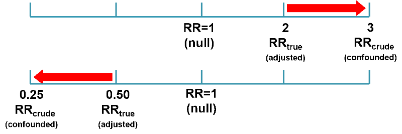
Confounding can bias the primary measure of association toward the null, causing an underestimate of the association. This is referred to as negative confounding. As illustrated below, if the true (adjusted) risk ratio or odds ratio was 3 and the crude, i.e., confounded estimate was OR or RR=2, that would be an underestimate. Similarly, if the true ratio was 0.25 (a preventive effect) and the crude estimate was 0.5, that would be an underestimate of the preventive effective.
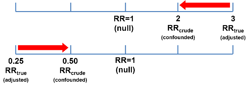
Confounding can also bias the measure of association away from the null, causing an overestimate of the association. This is called positive confounding. If the true odds ratio was 2 and the crude estimate was 3, that would represent an overestimate of the risk. And if the true odds ratio was 0.5 and the crude estimate was 0.25, that would also be bias away from the null and an overestimate of the preventive effect.
So, negative and positive confounding are distinguished not by whether it causes the measure of association to appear smaller or larger than the true value, but by whether it causes the estimated measure of association to move toward the null (negative) or away from the null (positive).
Down syndrome (trisomy 21) occurs when an individual is born with three copies of chromosome 21 instead of the normal two copies. The vast majority of these occur as a result of an error in meiosis during gamete formation, usually in oogenesis.
One can demonstrate that the frequency of Down syndrome increases with birth order, with a frequency of about 57 per 100,000 live births in 1st born children rising to about 164 per 100,000 in 5th born children.
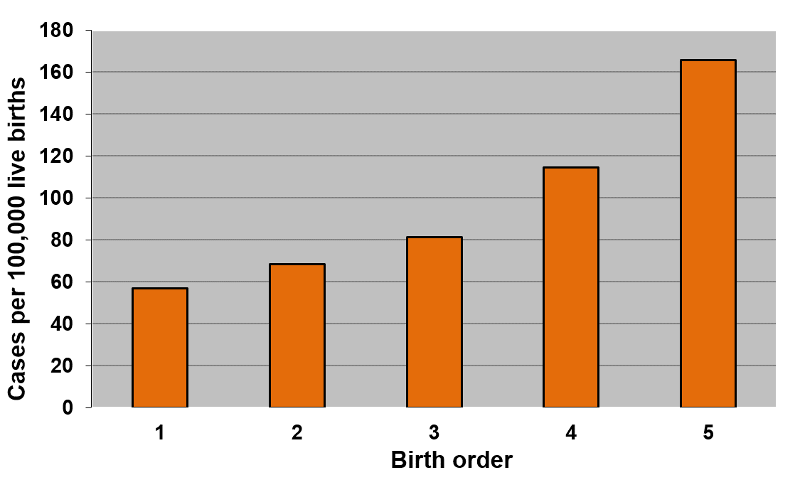
[Data and graphs adapted from Rothman K: Epidemiology: An Introduction using data from Stark CR and Mantel N: Effects of maternal age and birth order on the risk of mongolism and leukemia. J. Natl. Cancer Inst. 37(5):687-98, 1966]
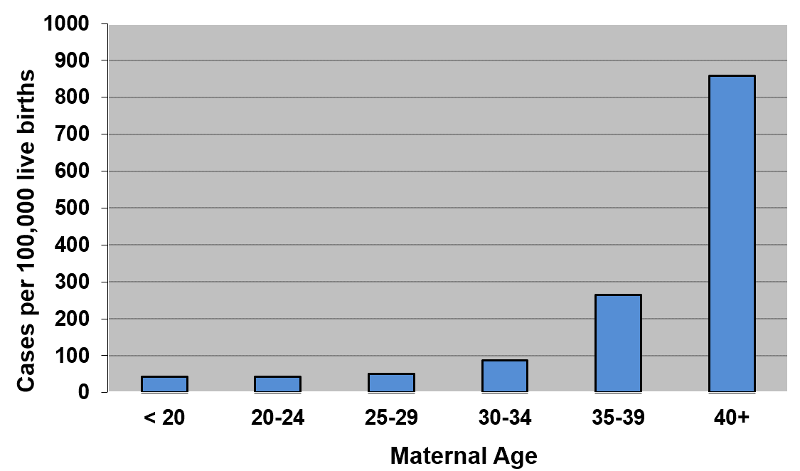
However, the frequency of Down syndrome also increases with maternal age, starting at about 40 per 100,000 live births in mothers under the age of 20 and rising slowly at first until age 35-39 when the frequency is about 270 per 100,000 live births, and then jumping to about 855 per 100,000 live births in mothers 40 years of age or older.
It is certainly not surprising that the increase with birth order correlates with the increase in maternal age. Mothers giving birth to their first born will have a younger age distribution than those giving birth to their 5th born. So, which matters? Birth order or maternal age? Is the association between birth order and Down syndrome confounded by maternal age? Or is the association between Down syndrome and maternal age confounded by birth order?
Stratifying the data by both birth order and maternal age, as in the three-dimensional bar graph below, clarifies this by showing the frequency of Down syndrome (on the vertical axis) stratified by both birth order (on the horizontal axis) and maternal age (on an axis projecting away from the reader). The figure shows that at any given maternal age, the birth order has little, if any, effect; the frequency of Down syndrome is low in young moms regardless of birth order, and the frequency of Down syndrome is high in older moms regardless of birth order.
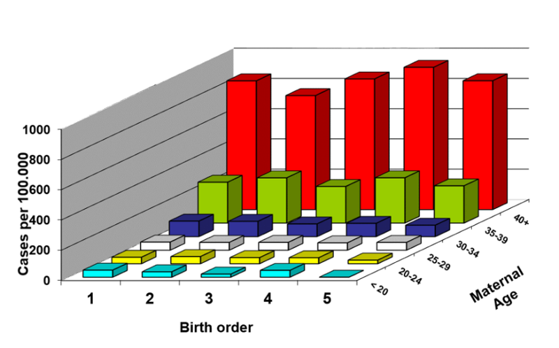
In other words, if we control for maternal age, birth order is not associated with prevalence of Down syndrome; it is not an independent risk factor. However, within each stratum of birth order, prevalence increases with maternal age, meaning that, controlling for birth order, the strong association with maternal age persists. Given our definition of confounding, the effect of birth order was confounded by maternal age, since maternal age made it appear that there was an association with birth order. However, when stratified by both birth order and maternal age, we can see that birth order did not have an independent effect. Its apparent association was totally the result of confounding and overestimation caused by maternal age.
Confounding is a major problem in epidemiologic research, and it accounts for many of the discrepancies among published studies. Nevertheless, there are ways of minimizing confounding in the design phase of a study, and there are also methods for adjusting for confounding during analysis of a study.
The ideal way to minimize the effects of confounding is to conduct a large randomized clinical trial so that each subject has an equal chance of being assigned to any of the treatment options. If this is done with a sufficiently large number of subjects, other risk factors (i.e., confounding factors) should be equally distributed among the exposure groups. The beauty of this is that even unknown confounding factors will be equally distributed among the comparison groups. If all of these other factors are distributed equally among the groups being compared, they will not distort the association between the treatment being studied and the outcome.
The success of randomization is usually evaluated in one of the first tables in a clinical trial, i.e., a table comparing characteristics of the exposure groups. If the groups have similar distributions of all of the known confounding factors, then randomization was successful. However, if randomization was not successful in producing equal distributions of confounding factors, then methods of adjusting for confounding must be used in the analysis of the data.
Limiting the study to subjects in one category of the confounder is a simple way of ensuring that all participants have the same level of the confounder. For example,
Restriction is simple and generally effective, but it has several drawbacks:
Another risk factor can only cause confounding if it is distributed differently in the groups being compared. Therefore, another method of preventing confounding is to match the subjects with respect to confounding variables. This method can be used in both cohort studies and in case-control studies in order to enroll a reference group that has artificially been created to have the same distribution of a confounding factor as the index group. For example,
Confounding is a type of bias, because it causes biased estimates of associations. However, confounding is different from selection bias and information bias, because it is caused by an imbalance in other risk factors, and the investigators can adjust for confounding in the analysis phase in order to minimize its effects. This is not true of selection bias or information bias; once they effect a study, there is no way to adjust for them. One can only try to figure out what effect they had on the estimate of effect.
However, if the investigators have collected data from their subjects regarding their status with respect to possible confounding factors, there are methods for computing adjusted measures of association. These are:
Analytic methods of adjustment attempt to determine how the groups would have compared if they had been comparable with respect to one or more confounding factors. As such, they provide an estimate of effect (association) that is closer to the truth.
Standardization is a method of computing and comparing adjusted rates of disease that indicate how the groups would have differed if they had had the same distribution of confounders.
To illustrate this we will consider a comparison of mortality rates in Florida and Alaska, two states with very different age distributions. Since older age is clearly a risk factor for death, a crude comparison of mortality rates will be confounded by differences in age.
| Florida | Alaska | |
|---|---|---|
| Total annual deaths | 131,902 | 2,116 |
| Total population | 12,340,000 | 530,000 |
| Crude mortality rate/100,000 | 1,069 | 399 |
The crude mortality rates are clearly different. The crude mortality ratio is 1069/399 = 2.68. Does this mean it is riskier to live in Florida?
The table below shows the age-specific mortality rates for Florida and Alaska. Two things are noteworthy. First, despite the difference in overall crude mortality rates, the age-specificmortality rates are quite similar. Second, besides the obvious difference in total population size, the big difference is in the age distribution of the two states. Florida has a larger proportion of older people (who have higher age-specific mortality rates) and Alaska has a greater proportion of younger people (who have lower age-specific mortality rates).
|
|
Florida |
Alaska |
||||
|
Age |
Population |
% of total (weight) |
Rate/100,000 |
Population |
% of total (weight) |
Rate/100,000 |
|
<5 |
850,000 |
7% |
284 |
60,000 |
11% |
274 |
|
5-19 |
2,280,000 |
18% |
57 |
130,000 |
25% |
65 |
|
20-44 |
4,410,000 |
36% |
198 |
240,000 |
45% |
188 |
|
45-64 |
2,600,000 |
21% |
815 |
80,000 |
15% |
629 |
|
>65 |
2,200,000 |
18% |
4,425 |
20,000 |
4% |
4,350 |
|
Totals |
12,340,000 |
100% |
530,000 |
100% |
||
As a result, the comparison of crude rates is unfair because Florida has a much larger proportion of older people who contribute heavily to the overall crude mortality rate in Florida. This comparison is clearly confounded by differences in age.
In essence, the crude mortality rate is a weighted average of the age-specific mortality rates for which the "weight" is the proportion of each population in a given age category. For example, if I multiply the proportion in each age category for Florida by the corresponding age-specific rate and add these up, I will get the crude mortality rate for Florida:
0.07(284) + 0.18(57) + 0.36(198) + 0.21(815) + 0.18(4425) = 1069
So, the crude rates are summary rates that indicate the weighted average of the age-specific rates.
The key question here is "How would the overall mortality rates have compared if the two populations had had the same age distribution?" If we could do this, we could compute an overall mortality rate that was unconfounded and more accurately reflected the similarity that we see in the age-specific rates in the two populations.
We can actually answer this question by using each state's observed age-specific rates and a single age distribution, i.e., a uniform set of "weights," meaning the proportion in each age category. By doing this, we can calculate hypothetical summary rates that are unconfounded by differences in age distribution, because we are applying the same age distribution to each state's observed age-specific rates. By doing this we can calculate adjusted overall summary rates that are no longer confounded by differences in age distribution.
To illustrate we will arbitrarily use the distribution of the United States population in 1988 as the standard set of weights. (We could use any other year, and it won't matter as long as we apply the standard set to both populations).
The age-distribution in the US in 1988 was:
| Age Category | Percent of Total Population |
|---|---|
| <5 | 7% |
| 5-19 | 22% |
| 20-44 | 40% |
| 45-64 | 19% |
| >65 | 12% |
Now let's use these weights to calculate age-adjusted rates, first for Florida, and then for Alaska.
Mortality Rate FL.adjusted = 0.07(284) + 0.22(57) + 0.40(198) + 0.19(815) + 0.12(4425) = 797/100,000
Mortality Rate Alaska.adjusted = 0.07(274) + 0.22(65) + 0.40(188) + 0.19(629) + 0.12(4350) = 750/100,000
These summary rates are hypothetical, but we can use them to provide a comparison of mortality rates that is not confounded by age.
Standardized Mortality Rate Ratio (SMR) = 797/750 = 1.06
Recall that the mortality rate ratio was 2.68, but now the standardized mortality rate ratio is 1.06, very close to the null value of 1.
Standardization is frequently used to generate "age-adjusted" rates not only for mortality, but for many other health outcomes in publications from CDC and in publications like Healthy People 2020. The image below shows heart disease deaths for black and white males and females in Massachusetts from 1970 to 1993. The footnote at the bottom says, "Rates are age-adjusted by the direct method using the 1940 U.S. population as a standard."

Having computed age-adjusted CHD death rates for each of these four sex and gender groups at multiple points in time, we get a clear picture of differences among the four groups and trends over time, and these comparisons are not distorted by the differences in age distribution among the groups over time. We can see clearly that CHD death rates have fallen in all four groups, but there are persistent large differences between males and females, even though the gap has narrowed somewhat. In addition, white females continue to have slightly lower CHD mortality rates than black femailes, and white males have slightly lower rates than black males.
A useful way to identify confounding is to calculate the crude (unadjusted) measure of association and then compute the measure of association again after adjusting for a possible confounding factor, as we did above. If the two differ, it suggests that the factor we adjusted for was a confounder. But how big a difference must there be to conclude that there was confounding?
Most epidemiologists use a 10% difference as a "rule of thumb" for identifying the presence of confounding. The magnitude of confounding is the percent difference between the crude and adjusted measures of association, calculated as follows (for either a risk ratio or an odds ratio):

If the % difference is 10% or greater, we conclude that there was confounding. If it is <10%, we conclude that there was little, if any, confounding.
For mortality rate ratios in Florida and Alaska:

Since 152% is much greater than 10%, the comparison of mortality rates was clearly confounded by differences in age distribution
Finally, note that the 10% rule of thumb for confounding is not rigid. Epidemiologists sometimes adjust for factors when the percent difference is less than 10%.
If age, for example, is a confounding factor when evaluating an association, another strategy is to evaluate the association in different age groups and calculate the measure of association in each stratum of age.
For example, if age is a confounder of the relation between physical activity and CHD, we could stratify the analysis into separate age groups in order to evaluate the association between activity and CHD separately for each age group. The table below shows a hypothetical example.
| CHD | No CHD | Total | |
|---|---|---|---|
| Active | 48 | 800 | 848 |
| Not active | 69 | 625 | 694 |
The crude risk ratio is (48/848) / (69/694) = 0.57.
If we are concerned about confounding by age, we could restrict the analysis to young subjects (arbitrarily defined as less than 45 years of age), or we could restrict it to older subjects (45 years or older). However, a better option would be to enroll young and old subjects, but analyze them separately, i.e., a stratified analysis. To do this we need to have recorded each subjects age, i.e., we need to have data on confounding factors, and, since age is continuously distributed, we need to collapse ages into categories. For the sake of illustration, we will collapse age into just two categories here, although breaking the data into five year intervals would give better control of confounding.
The stratified analysis might look like this with younger subjects on the left and older subjects on the right:
|
|
Younger (<45) |
Older (≥45) |
||||||
| CHD | No CHD | Total | CHD | No CHD | Total | |||
| Active | 25 | 600 | 625 | Active | 23 | 200 | 223 | |
| Not active | 11 | 225 | 236 | Not | 58 | 400 | 458 | |
RRyoung = 0.86 RRold = 0.81
Notice that when the data is stratified this way, it becomes apparent that most of the young subjects were active, and most of the older subjects were not. By stratifying the analysis in this fashion, we have reduced confounding by disentangling the effects of activity and age. The contingency table for the young shows the effect of activity on CHD risk in the young without the additional risk factor of older age. Similarly, the analysis of the older subjects shows the effect of activity on CHD risk in the older group without the inclusion of younger people whose inherent risk of CHD is less.
Also notice that the stratum-specific risk ratios are similar to one another, although both are less than the crude risk ratio. Therefore, the effect of activity in reducing the risk of CHD is similarly in both age groups, but the effect is not as strong as the crude risk ratio suggested.
The analysis above stratified by age into only two groups for simplicity. However, using just two broad ranges of age would probably result in residual confounding, because the age-related risk of CHD might vary quite a lot between the ages of 45-80 in the older group. Better control of confounding could be achieved by stratifying more finely, perhaps at five year intervals of age.
Residual confounding is confounding that persists despite efforts to control or adjust for confounding. There are several causes for residual confounding:
When the stratum-specific estimates of effect (RR or OR) are similar, as in the example above, one can combine them into a single summary measure of association that is adjusted for confounding by the stratified variable. This is most commonly done using a Mantel-Haenszel equation to compute a weighted average, i.e., a pooled estimate of the stratum-specific risk ratios (or odds ratios). The adjusted estimate is often reported as RRMH or ORMH (i.e., an adjusted measure of association). For the example, above,
RRMH=0.84
[Note: You will not need to compute Mantel-Haenszel estimates in this course, but you will be expected to interpret them.]
With a pooled estimate we can now compute the magnitude of confounding as we did in the discussion of standardization.
For Activity and CHD:

The crude estimate of the risk ratio and the adjusted estimate differed by 32%. Using the 10% rule for confounding, we can conclude that there is clear evidence of confounding by age.
|
Stratified analysis is a straightforward and effective way to control for confounding. Its chief limitation is that it cannot effectively control for confounding by multiple variables simultaneously, because stratifying by additional layers for each confounder is limited by sample size. Multiple variable regression is a better method for controlling for multiple confounding factors simultaneously, but a series of stratified analyses stratified one possible confounder at a time is a good way to get a sense of which other factors might cause confounding (or effect measure modification) prior to embarking on multiple variable regression (Effect Measure Modification is explained on page 8).
|
We also could have computed a risk ratio adjusted for confounding by age using standardization. In the table below the data has been rearranged to facilitate this.
|
Physically Active |
Sedentary |
|||||||||
| CHD | Population | % pop. | Rate | CHD | Population | % pop. | Rate | |||
| Young | 25 | 625 | 0.737 | 0.0400 | Young | 11 | 236 | 0.340 | 0.0466 | |
| Old | 23 | 223 | 0.263 | 0.1031 | Old | 58 | 458 | 0.660 | 0.1266 | |
| TOTAL | 48 | 848 | 1 | 69 | 694 | 1 | ||||
Note that only 26.3% of the "active" population is old, but 66% of the inactive population is old, and old subjects have more than 2 times the risk of CHD compared to the young subjects.
I can use the proportions of young and old subjects in the physically active group as standard weights and apply these proportions to the sedentary group to compute an adjusted rate for the sedentary group that estimates what their overall rate would have been if their age distribution had been the same as the active group.
CHD Rate active adj.=0.737(0.04)+0.263(0.1031)=0.0566
CHD Rate sedentary adj.=0.737(0.0466)+0.263(0.1266)=0.0678
Adjusted Risk Ratio = 0.0566/0.0678 = 0.837, essentially the same value when the Mantel-Haenszel equation was used.
Confounding by indication is a special type of confounding that can occur in observational (non-experimental) pharmaco-epidemiologic studies of the effects and side effects of drugs. This type of confounding arises from the fact that individuals who are prescribed a medication or who take a given medication are taking it for a reason, and they are inherently different from those who do not take the drug. In medical terminology, those who take the drug have an "indication" for use of the drug. Even if the study population consists of subjects with the same disease, e.g., osteoarthritis, they may differ in the severity of their disease and may therefore differ in the need for medication. Aschengrau and Seage give the example of studies of the association between antidepressant drug use and infertility. The use of antidepressant medications may appear to be associated with an increased risk of infertility. However, depression itself is a known risk factor for infertility. As a result, there would appear to be an association between antidepressants and infertility. One way of dealing with this is to study the association in subjects who are receiving different treatments for the same underlying disease condition.
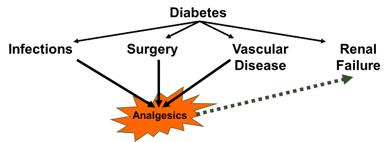
A variation on this might be dubbed "confounding by contraindication." Perneger and Whelton conducted a population-based case-control study to examine the association between analgesic drug use and kidney failure. The authors compared prior analgesic use between patients receiving kidney dialysis and population controls without known kidney disease. Suppose that patients on dialysis had been advised to avoid taking aspirin because of its effects on blood clotting; they may have been advised to take acetaminophen (Tylenol) instead). If the group of dialysis cases included a number of people who had been on long-term dialysis, this would result in a decreased frequency of aspirin use and increased use of Tylenol in the case group. As a result, an association with aspirin would be underestimated, while an association with Tylenol would be overestimated.
Reverse causality occurs when the probability of the outcome is causally related to the exposure being studied. For example, Child feeding recommendations of the World Health Organization include breastfeeding for two years or more, because of evidence that breast fed children have a reduced risk of infectious agents and are less likely to die. However, some studies have produced conflicting concerns. One possibility is that in communities with very poor resources the children who are at greatest risk and perhaps have the least access to other food sources are more likely to be breast fed for at least two years. A comparison of growth and development between these children and more advantaged children would likely find less progress in the breast fed group. (See "Association of Breastfeeding and Stunting in Peruvian Toddlers: An Example of Reverse Causality" by Marquis GS, et al.: International Journal of Epidemiology 1997; 26: 349-356).
The case-control study by Perneger and Whelton, mentioned above, may also have been affected by reverse causality. Diabetes is a leading cause of renal failure in the US, and chronic diabetes is associated with a number of other health problems such as cardiovascular diseases and infections that could result in a greater use of analgesics. If so, the dialysis cases whose renal failure resulted from diabetes might have taken more analgesics because of their diabetes. Nevertheless, it would appear that analgesic use was associated with an increased risk of renal failure rather than vice versa.
In the example looking at the association between physical activity and CHD we noted that the risk ratio was 0.86 in the younger subjects and 0.81 in the older subjects. The similarity indicates that the effect of physical activity on CHD was simiar in both age groups. But what if the risk ratios had been meaningfully different?
Consider the following reports. The American Journal of Family Medicine contained an article describing an unusual neurological syndrome (Reyes syndrome) that developed shortly after a viral illness in 12 subjects. All 12 had taken aspirin during their viral illness, and the author hypothesized that this was a new syndrome of toxicity to aspirin. After the publication of this small case series, the CDC issued a bulletin and asked for reports of similar neurological problems after a viral illness. The responses stimulated a second study based on 64 subjects with the same neurological problems after a viral illness and a comparison group consisting of 17,000 subjects who had had a viral illness but did not have Reyes syndrome.
|
Crude Analysis |
||
|
Reyes |
No Reyes |
|
|
Aspirin |
57 |
8500 |
|
No aspirin |
7 |
8500 |
|
Total |
64 |
17000 |
ORcrude = 8.14
Since most of the cases had been children, the investigators performed a stratified analysis to examine the association between aspirin and Reyes syndrome separately in children and adults.
|
|
Children |
|
|
Adults |
||
|
Reyes |
No Reyes |
|
|
Reyes |
No Reyes |
|
|
Aspirin |
52 |
2500 |
|
Aspirin |
5 |
6000 |
|
No aspirin |
3 |
1000 |
|
No aspirin |
4 |
7500 |
|
Total |
55 |
3500 |
|
|
9 |
13,500 |
ORchildren = 6.93 (2.16-22.25) ORadult = 1.56 (0.42-5.82)
In this case, the association between aspirin use after a febrile illness and development of Reyes syndrome is clearly different in children and adults. This phenomenon is called effect measure modification, but unlike confounding, this is not a mathematical distortion; it is a difference in the response to aspirin in these two age groups. Effect measure modification is not a bias or error, and it is not something that we need to avoid or adjust for. It is just an interesting observation that the measure of association differs across groups.
Effect measure modification simpley means that two or more stratum-specific estimates are different. In other words, the association between an exposure and a disease differs among groups of people. For example, we know that the the relative risk of CHD is higher in males than in females.
Consider another example. Trauma surgeons at Boston City Hospital used their trauma database to look at risk factors for death in automobile drivers who had been injured severely enough to require hospital admission after a collision. Not surprisingly, drivers over the age of 70 had a much higher risk of dying after admission compared to yournger drivers who had been admitted (risk ratio=6.75), even after adjusting to differences in severity of injury. When the data were stratified into unrestrained drivers and those who had worn a seatbelt or had a functioning air bag, the following results were obtained.
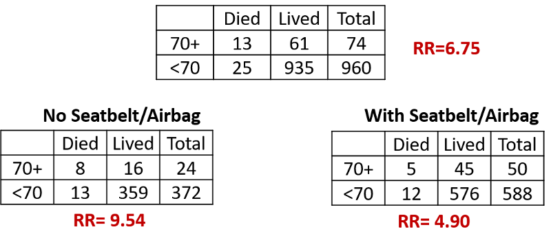
The risk ratio for the association between age and mortality 9.54 in unrestrained drivers and 4.90 in drivers with seatbelts or airbags. Drivers over 70 years of age had a greater risk of dying compared to younger drivers in both subsets, but the association was twice as strong when a seatbelt or airbag was not used.
Rather than obscuring this difference in effect by computing a Mantel-Haenszel pooled estimate, one should report the two effects separately, because it is of scientific interest and to identify subsets of the population that are particularly susceptible (more likely to develop adverse effects).
Having said that, be aware that effect measure modification and confounding can both be present. To evaluate that possibility, one can compute a Mantel-Haenszel pooled estimate for the purpose of determining whether confounding was also present. In this case,
ORMH = 4.48
We can use this pooled estimate to compute the magnitude of confounding:
For aspirin use after a febrile illness and Reyes' syndrome:

So there was both effective measure modification by age and confounding by age in this study.
In this example, there was an obvious difference in the stratum-specific odds ratios, but sometimes there are smaller differences. Unfortunately, the 10% rule for confounding does not apply to determining whether there is effect measure modification. This is a complex area that is beyond the scope of this course. For our purposes, you must make a judgment regarding whether an observed difference in effect is "meaningful" and whether it is plausibly due to a biological phenomenon.
While the main focus of a study may to evaluate the association between a particular exposure and a particular health outcome, attention must be given to other risk factors that might cause confounding or effect measure modification. Even if they are not of primary interest other risk factors can have several possible effects.
Stratification is a useful tool for
Steps in Stratified Analysis
 Test Yourself
A study was conducted to examine the association between smoking and oral cancer in patients who had been previously treated for thyroid cancer. Some of the patients with thyroid cancer had been treated with radiation and some had been treated surgically without radiation. The crude risk ratio for smoking and oral cancer was 2.3. A stratified analysis showed RR=4.8 in those who had been radiated and RR=2.2 in those who had not. The Mantel-Haenszel pooled estimated was RRMH=2.5. Was there evidence of confounding or effect measure modification?
Answer
Test Yourself
A prospective cohort study was conducted to evaluate the association between regular exercise and obesity. The crude incidence rate ratio (IRR) for regular exercisers compared to non-exercisers was 0.78. When stratified by diet (healthy diet versus unhealthy diet), the IRR in healthy eaters was 0.54, and the IRR for unhealthy eaters was 0.85. The Mantel-Haenszel pooled estimate was RRMH=0.62. Was there evidence of confounding or effect measure modification?
Answer
Test Yourself
Interpret the diet-adjusted incidence rate ratio in the previous question.
Answer
Test Yourself
In the question above on the association between exercise and obesity, interpret the incidence rate ratio for the association of exercise and obesity among healthy eaters.
Answer