Standardized Rates of Disease
When comparing two or more populations with respect to a health outcome, it is temptiing to compare crude rates of disease, i.e., the number of disease events divided by the size of the population. The "crude rate" is the measure that was introduced in the module on Measures of Disease Frequency. However, comparisons of crude rates can be misleading because of confounding if the populations being compared have different distributions of other determinants of disease, such as age which has an important effect on many heatlh outcomes, such as mortality, heart disease, cancer, infectious diseases, and injury. As a result, differences in age can distort other comparisons between populations, and this distortion is called confounding. This module will focus on a technique called standardization that allows one to compute summary rates of health outcomes that are adjusted to take into account differences in confounding factors like age in order to provide a less distorted comparison.
The two closely related techniques are commonly used to compute "age-adjusted" summary rates that facilitate compartisons among population. Direct standardization applies a standard age distribution to the populations being compared in order to compute summary rates indicating how overall rates would have compared if the populations had had the same age distibution. This method is used when age-specific rates of disease are known for the populations being compared. In contrast, so-called indirect standardization applies a standard set of age-specific rates of disease to the populations being compared in order to compute the number of cases of disease that would be expected in a given population, based on its size and age-distribution.
After completing this module, the student will be able to:
Crude rates
Age-specific rates
Standardized rates

Crude rates are quite simple and straightforward. They are calculated by dividing the total number of cases in a given time period by the total number of persons in the population. In this case Population B has a higher crude rate of disease. If we think about these two populations as the 'exposures' of interest, does this imply that it is riskier to live in Population B compared to Population A?
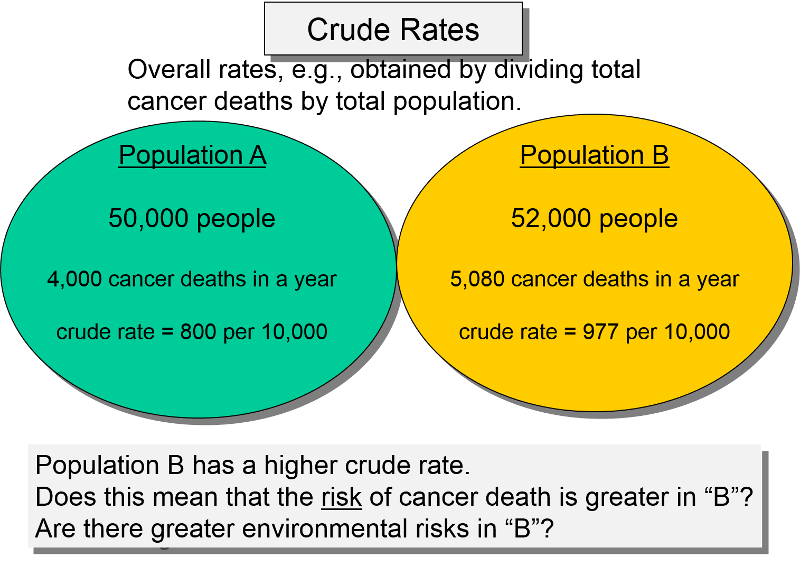
The problem with this comparison is that the crude rate is an overall average rate of disease, but it doesn't take into account possible confounding factors.
A confounding factor is basically another risk factor for the outcome of interest that is also unequally distributed among the populations being compared. In this case, age is clearly an independent risk factor for cancer mortality, but what we really would like to know is whether there are differences in cancer mortality between the two populations that are not due to age differences, i.e., differences in mortality that are independent of age differences. If the two populations have unequal age distribution, it will distort the comparison of interest.
For example, Population B might have a greater percentage of older people, and we know that the risk of cancer mortality increases with age regardless of one's environment. If so, then the risk of death due to cancer in Population B might only appear to be greater simply because it has a greater percentage of old people who have an inherently greater risk of dying. In other words, the crude mortality rate for population B might be higher just because it is weighted more heavily with old people. In this setting we might be interested in comparing the mortality rates without the unwanted confounding effect of age.
This problem is clearer if we take a more detailed look by examining the age-specific mortality rates within each of these populations, as shown below.
In this hypothetical example, the table below shows that the age-specific mortality rates are absolutely identical in the two populations. In other words, in any given age group, the two populations have the same risk. However, note that the risk of mortality increases with age. Note also that Population B has a greater percentage of older people. In other words, population B is more heavily weighted with older people, and age is also associated with risk of mortality, so the comparison of crude rates is unfair, because of the unequal age distributions.
Table - Population A
|
Age Group |
Number of Deaths |
Number of People |
Death Rate per 10,000 |
|---|---|---|---|
|
30-39 |
400 |
10,000 |
400 |
|
40-49 |
600 |
10,000 |
600 |
|
50-59 |
800 |
10,000 |
800 |
|
60-69 |
1,000 |
10,000 |
1,000 |
|
70-79 |
1,200 |
10,000 |
1,200 |
|
Totals |
4,000 |
50,000 |
800 |
Table - Population B
|
Age Group |
Number of Deaths |
Number of People |
Death Rate per 10,000 |
|---|---|---|---|
|
30-39 |
80 |
2,000 |
400 |
|
40-49 |
300 |
5,000 |
600 |
|
50-59 |
800 |
10,000 |
800 |
|
60-69 |
1,500 |
15,000 |
1,000 |
|
70-79 |
2,400 |
20,000 |
1,200 |
|
Totals |
5,080 |
52,000 |
977 |
Since the age-specific rates are identical, the risk of cancer mortality is exactly the same in these two populations. What makes the crude rates different is that older people have a higher risk of cancer mortality, and population B has a greater proportion of older people. In other words, the age-specific rates are the same, but the higher proportion of older people in population B means that the overall crude rate is more heavily weighted by the age-specific rate among older people.
This method, sometimes referred to as direct standardization, provides a useful way to compare health outcomes among populations that may have different age distributions. This is done by applying a standard age distribution to the populations being compared in order to compute hypothetical summary rates indicating how the overall rates would have compared if the populations had had the same age distibution. This method is used when age-specific rates of disease are known for the populations being compared.
This table summarizes the data used to calculate crude (unadjusted) rates for Florida and Alaska. Note that the crude rate for Florida is substantially greater than Alaska's, raising the possibility that it is riskier to live in Florida. Are there social, behavioral, or environmental factors that account for the higher mortality rates? Is the risk of death really greater in Florida?
|
Florida |
Alaska |
|
|---|---|---|
|
Number of deaths |
131,902 |
2,116 |
|
Total population |
12,340,000 |
530,000 |
|
Crude mortality rate (per 100,000) |
1,069 |
399 |
Note also that the crude mortality rate ratio is 1,069/399 = 2.68. However, as you probably know, many older people move to Florida when they retire, so the population of Florida contains a higher percentage of older people, and they have an inherently greater risk of dying compared to young people. As a result, comparing the crude rates is likely to be misleading about whether the risk of death is truly greater in Florida. This is illustrated in detail in the table below.
Table - Age-specific Mortality Rates in Florida
|
Age Group |
Number of People |
% of Total Pop. |
Death Rate per 100,000 |
|---|---|---|---|
|
<5 |
850,000 |
7% |
284 |
|
5-19 |
2,280,000 |
18% |
57 |
|
20-44 |
4,410,000 |
36% |
198 |
|
45-64 |
2,600,000 |
21% |
815 |
|
>64 |
2,200,000 |
18% |
4,425 |
|
Totals |
12,340,000 |
100% |
1,069 (crude rate) |
Table - Age-specific Mortality Rates in Alaska
|
Age Group |
Number of People |
% of Total Pop. |
Death Rate per 100,000 |
|---|---|---|---|
|
<5 |
60,000 |
11% |
274 |
|
5-19 |
130,000 |
25% |
65 |
|
20-44 |
240,000 |
45% |
188 |
|
45-64 |
80,000 |
15% |
629 |
|
>64 |
20,000 |
4% |
4,350 |
|
Totals |
530,000 |
100% |
399 (crude rate) |
When we look at the age-specific mortality rates, we see that there is little difference within each age group, certainly nothing like the approximately 2.7 (1069/399) times higher crude death rate in Florida than in Alaska . In theory, we could simply report the age-specific rates and let people compare different states by looking at the rates within each age group separately, but that is less than ideal for two reasons. First, if we wanted to look at all of the 50 states side-by-side, it would be extremely difficult to compare by looking at all the age-specific rates in each state. More importantly, looking at the age-specific rates doesn't necessarily tell us whether one state is higher than another and certainly not the size of any difference. What we would like is a single summary rate like we have with the crude rate, but with the distortion caused by age removed. This is what standardization accomplishes.
In order to understand how this works, it is helpful to take another look at the crude rate.
Method #1: The simple, logical way to calculate the crude death rates is to divide the total events by the total population.
(total # deaths / total population) = (131,902 / 12,340,000 = 0 .01069 = 1,069 / 100,000 population
Method #2: The Long Way to Calculate the Crude Rate (Just to make a teaching point)*
If asked to compute a crude rate, the sensible thing would be to use method #1. However, it is also possible to calculate the crude rate by multiplying the age-specific rates by the fraction of the population that they represent and then summing this up. The "weight" of each age category is given by the fraction of the total population that it represents. For example, the "weight" of the youngest age group in Florida is 0.07 or 7%, while the weight of the oldest age group in Florida is 0.18, or 18%.
So, in the example above, we could calculate the crude rate for Florida as:
(.07) x (284/100,000) = 19.88/100,000
+ (.18) x (57/100,000) = 10.26/100,000
+ (.36) x (198/100,000) = 71.28/100,000
+ (.21) x (815/100,000) = 171.15/100,000
+ (.18) x (4,425/100,000) = 796.25/100,000
Total = 1,069 /100,000 population
NOTE: This is a laborious way to calculate the crude rate; it makes much more sense to just divide the total number of deaths by the total population size. However, we are doing this the long way just to illustrate that if you weight the category-specific rates according to the proportion of the population in each group and then add them, you end up with the crude rate. Because of this, even if two populations have identical category-specific rates, the crude rates will vary if the distributions of the populations are different.
As noted above, age-specific rates provide a fairer comparison, but in many situations it is useful to have any overall summary rate that is adjusted for a confounding factor like age, so you can easily compare multiple populations. This can be done be calculating an "adjusted" overall rate which provides for a fairer comparison. In essence, this is accomplished by asking the question "How would the rates have compared if the two populations had had the same age distribution?" I will illustrate how to do this when comparing two populations, but keep in mind that multiple populations can be "adjusted" this way.
The Question We Would Like to Answer:
"What would the comparable death rate be in each state if both populations had identical age distributions?"
We saw above that the crude rate is a weighted average, but the comparison is distorted if the populations have different age distributions. In order to see how the two population would have compared if they had had the same distribution, we can calculate a summary rate by pretending that the distributions are the same in the populations being compared. We will use the long method of calculating the summary rate, as show at the bottom of the previous page. We will use each population's actual age-specific rates, BUT we will apply the same set of weights (fraction of people in each age group) to all of the populations being compared. In essence, this will give us a summary rate that is adjusted in a way that answers the question posed in the table above.
Basically, an age-standardized rate is also a weighted average, but the weights for the age categories are artificially set to be equal for the populations being compared by applying the weights of some standard population to each of them. We are still using the actual age-specific rates of each of the populations, but we are weighting them using a uniform standard population distribution.
What age distribution should you use? It doesn't really matter, but you usually see one of the following used for a standard age-distribution:
Example #1: Calculating standardized Rates using Florida's age distribution as the standard
If I wanted to ask the question "What would Alaska's overall mortality rate have looked like if Alaska had its actual age-specific rates but also had the same age distribution in the population as Florida?" I can do this quite simply by applying Florida's population distribution to Alaska's age-specific rates.
First, we will calculate the standardized rate for Florida by multiplying each of Florida's age-specific rates by the fraction of the Florida's population in each age group.
For the age group <5 years old: 0.07 x 284 = 19.18
For the age group 5 to 19 years: 0.18 x 57 = 10.26
For the age group 20 to 44 years: 0.36 x 198 = 71.28
For the age group 45 to 64 years: 0.21 x 815 = 154.85
For the age group greater than 64 year: 0.18 x 4,425 = 796.50
SUM = 1069 per 100,000 population
As you would expect, the standardized rate in Florida is the same as its crude rate, because we used Florida's age distribution as the standard.
Now let's use Florida's age distribution as the standard to calculate Alaska's standardized rate by multiplying each of Alaska's age-specific rates by the fraction of the Florida's population in each age group.
For the age group <5 years old: 0.07 x 274 = 19.18
For the age group 5 to 19 years: 0.18 x 65 = 11.70
For the age group 20 to 44 years: 0.36 x 188 = 67.68
For the age group 45 to 64 years: 0.21 x 629 = 132.09
For the age group greater than 64 year: 0.18 x 4,350 = 783.00
SUM = 1014 per 100,000 population
We can compare Florida's standardized rate to Alaska's standardized rate by computing a standardized rate ratio (SRR) = 1069/1014 = 1.054, much less than the crude mortality rate ratio of 2.68, suggesting that much of the crude difference was due to confounding by age.
In this example we adjusted for age differences by using Florida's age distribution as a standard set of weights and applied those weights to the age-specific rates of each state. However, we could have achieved a fair comparison by using other standards as well, as long as we applied the same standard or weights to each of the populations being compared. For example, I could have arbitrarily chosen to use the age distribution of the US population in 1988 as the standard, as demonstrated on the next page.
Example #2: Calculating Age-adjusted Rates Using an External Age Distribution as the Standard (e.g., using the age distribution of the US population in 1988 as the standard age distribution.)
Table - Distribution of the US Population in 1988
|
Age Group |
Population (% of Total) |
|---|---|
|
<5 |
18,300,000 (7%) |
|
5-19 |
52,900,000 (22%) |
|
20-44 |
98,100,000 (40%) |
|
45-64 |
46,000,000 (19%) |
|
>64 |
30,400,000 (12%) |
|
Total |
245,700,000 (100%) |
Now, let's use the US population distribution in 1988 as the standard distribution for both Florida and Alaska:
Here are the age-specific death rates for Florida and Alaska:
|
Age Group |
Florida Death Rates per 100,000 |
Alaska Death Rates per 100,000 |
|---|---|---|
|
<5 |
284 |
274 |
|
5-19 |
57 |
65 |
|
20-44 |
198 |
188 |
|
45-64 |
815 |
829 |
|
>64 |
4425 |
4350 |
First, we will calculate the standardized rate for Florida by multiplying each of Florida's age-specific rates by the fraction of fraction of the age group in the standard population.
For the age group <5 years old: 0.07 x 284 = 19.88
For the age group 5 to 19 years: 0.22 x 57 = 12.54
For the age group 20 to 44 years: 0.40 x 198 = 79.20
For the age group 45 to 64 years: 0.19 x 815 = 154.85
For the age group greater than 64 year: 0.12 x 4,425 = 531.00
SUM = 797 per 100,000 population
Therefore, using the 1988 US population distribution as the standard, the standardized rate in Florida is 797 per 100,000 population, calculated.
Now let's use the standard population distribution to calculate Alaska's standardized rate by multiplying each of Alaskaa's age-specific rates by the fraction of fraction of the age group in the standard population.
For the age group <5 years old: 0.07 x 274 = 19.18
For the age group 5 to 19 years: 0.22 x 65 = 14.30
For the age group 20 to 44 years: 0.40 x 188 = 75.20
For the age group 45 to 64 years: 0.19 x 629 = 119.51
For the age group greater than 64 year: 0.12 x 4,350 = 522.00
SUM = 750 per 100,000 population
Using the 1988 US population distribution as the standard, the standardized rate in Alaska is 750 per 100,000 population, calculated by multiplying each of Alaska's age-specific rates by the fraction of fraction of the age group in the standard population.
Using the 1988 US population distribution as the standard gives different adjusted rates than when we used Florida as the standard, but the difference between the two states is almost identical to when we used Florida as the standard. Once again, note that the standardized rate ratio (SRR) = 797/750 = 1.06, i.e., much less than the crude mortality rate ratio of 2.68, but very close to the standardized rate ratio that was obtained when the age distribution of Florida was used as the standard.
These adjusted rates are hypothetical death rates that would have occurred in each state if each had the age distribution of the entire US population in 1988. It is important to note the the adjusted rates are artificial, because they are based on a hypothetical situation, and what one gets for the summary rates depends, to some extent, on what one selects as the standard. However, the more important observation is the impact on the comparison between the two populations. Both sets of weights provided age-standardized rates that showed there is little difference in mortality risk between the two states after adjusting for age.
Because rates can be compared only when weights are the same for each entity, basic public health data almost always use an external population to facilitate comparison with other entities. For example, to compare the mortality rates among all 50 U.S. states, it would make much more sense to use the U.S. population as a whole for the weights than weighting each state's population to Florida or any other state. This consideration carries over to the situation in which only two states are compared, or even when tracking trends over time in a single state, especially if over a time period long enough to see a change in the age distribution of the population.
Therefore, one would be much more likely to see a comparison between Florida and Alaska where the U.S. population was used as the standard (Example #2) than where the population of Florida was used (Example #1). Analogously, mortality rates among all the countries in the world typically use a world standard based population.
Currently, the age distribution of the population based on the 2000 Census is used for almost all measures in the United States, while the World Health Organization (WHO) has developed a standard population based on the average age distribution of the world's population
Standardized Rate Ratio
Standardization results in "adjusted" rates that are not real, but they have the advantage of enabling you to compare two or more populations after removing the distorting effect of other confounding factors, such as age. In many public health circumstances, it is important to compare rates of disease among two or more populations, but there may be differences in the distributions of the populations that distort the comparison. In this situation you will frequently see adjusted or standardized rates.
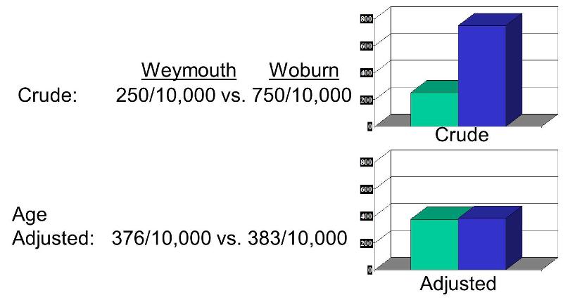
A comparison of crude and adjusted rates also provides a way to identify whether a factor is causing confounding. By definition, if you adjust for a factor like age and the relationship changes, then there was confounding. In the illustration below, Woburn's crude rate was 750 per 10,000 compared to Weymouth's crude rate of 250 per 10,000, a 3-fold difference. However, the age-adjusted rate for Woburn was 383 per 10,000, and the age-adjusted rate for Weymouth was 376 per 10,000. This indicates that the crude comparison was confounded by age.
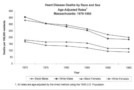
One might ask "Why not just compare the age-specific rates?" The answer is that there are times when unconfounded summary rates are very useful. For example, suppose you wanted to examine trends in mortality rates for heart disease over time, and you wanted to also see how trends compared among black and white males and females. In this situation you might have age-, race-, and gender-specific rates at multiple time points in a single population. However, there would be so many category-specific rates that it would be impossible to keep track of all of the comparisons and make any sense out of what was going on, as illustrated in the following tables showing age-, gender-, and race-specific rates of mortality from heart disease over time.
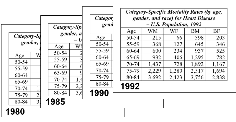
Trying to make sense out of all of these category-specific rates would be extremely difficult. On the other hand, if you calculated age-adjusted summary rates for black and white males and females for each year, you could then summarize these with a graph that allowed you to quickly see what the trends were, as illustrated below.
The video below provides a 20 min overview of standardized rates.
To calculate age-adjusted standardized rates, as above, one must first have the age-specific rates of disease for each of the populations to be compared. One then uses a standard age distribution to compute a hypothetical summary rate that indicates what the overall rate of disease would be for each population, if they had had the same age distribution as the standard. In other words, one uses each population's real age-specific rates and applies these to a single standard age distribution. In some situations, however, the age distribution of the populations being compared is know, but it is difficult, if not impossible, to obtain reliable estimates of age-specific rates, particularly if one is interested in smaller populations in which age-specific rates would be subject to random error because of relatively small numbers of observations. Consider the problem of a cluster of cancer cases that come to our attention in a specific community. The obvious question is whether the occurrence of cancer in this community is higher than that of other communities in the same state. However, the number of cases of a particular type of cancer occurring in even a relatively large community is typically small enough to produce very unstable rates due to random error. On the other hand, age-specific rates for the entire state would be much more stable, because of the larger sample size. In this situation one can approach the problem by using the age-specific rates observed for the entire state population as an estimate of the expected rates for the component communities. One can then apply these rates to the age distribution of each community to compute the expected number of specific cancer cases for a given community and then compare the expected number of cases to the observed cases. This approach is typically used by state cancer registries. Since the frequencies of different cancers oftern differ by gender, separate computations are performed for men and women.
Consider the following example adapted from the Massachusetts Department of Public Health:
|
Age Group |
A) Overall Age-specific State Rate |
B) Town's Population Size |
C) Expected Cases (A x B) |
Observed # of Cases |
|---|---|---|---|---|
|
0-19 |
0.0001 |
74,857 |
7.47 |
11 |
|
20-44 |
0.0002 |
134,957 |
26.99 |
25 |
|
45-64 |
0.0005 |
54,463 |
27.23 |
30 |
|
65-74 |
0.0015 |
25,136 |
37.70 |
40 |
|
75-84 |
0.0018 |
17,012 |
30.62 |
30 |
|
85+ |
0.0010 |
6,337 |
6.34 |
8 |
|
Totals |
136.35 |
144 |
SIR = (Observed Cases/Expected Cases) x 100 = (144/136.35 4) x 100 =106
Consequently, these results suggest that, after adjusting for age differences, the incidence of this particular type of cancer in this town was 6% higher than expected based on average age-specific rates for the state. The Massachusetts Department of Public Health provide the following comments regarding the limitations of thise type of data:
"... apparent increases or decreases in cancer incidence over time may reflect changes in diagnostic methods or case reporting rather than true changes in cancer incidence. Three other limitations must be considered when interpreting cancer incidence data for Massachusetts cities and towns: under-reporting in areas close to neighboring states, under-reporting of cancers that may not be diagnosed in hospitals, and cases being assigned to incorrect cities/towns."
Another important consideration is the precision of these estimates. This is best evaluated by computing a 95% confidence interval for the SIR. The Epi_Tools.XLS spreadsheet has a worksheet that will help you compute the confidence interval. For this example, the 95% confidence interval is:
95% confidence interval = 88 to123


One of the important applications of standardized incidence ratios is to monitor the frequency of cancer and other diseases. SIRs are partcularly useful because the number of any particular type of cancer cases is likely to be small in an individual town, particularly if the community is small. In this situation standardized rates are less useful since the age-specific rates for a particular cancer would be subject to a huge amount of random error due to the small number of cases. SIRs get around this problem hy using the more stable rates for the entire state in order to compute the expected number of cases of a given cancer for a community, given the community's age distribution.
In the video below Professor Richard Clapp, the first director of the Massachusetts Cancer Registry discusses the need for registries of this type.
The link below will take you to the website for the Massachusetts Cancer Registry, where you can explore the SIRs and confidence intervals for specific types of cancers throughout Massachusetts.
http://www.mass.gov/eohhs/gov/departments/dph/programs/health-stats/cancer-registry/
When the outcome of interest is a mortality rate, a standardized incidence ratio is referred to as a standardized mortality rate.