

Relationship of Incidence Rate to Cumulative Incidence (Risk)
Cumulative incidence (the proportion of a population at risk that will develop an outcome in a given period of time) provides a measure of risk, and it is an intuitive way to think about possible health outcomes. An incidence rate is less intuitive, because it is really an estimate of the instantaneous rate of disease, i.e. the rate at which new cases are occurring at any particular moment. Incidence rate is therefore more analogous to the speed of a car, which is typically expressed in miles per hour. Time has to elapse to measure a car's speed, but we don't have to wait a whole hour; we can glance at the speedometer to see the instantaneous rate of travel. Rather than measuring risk per se, incidence rate measures the rate at which new cases of disease occur per unit of time, and time is an integral part of the calculation of incidence rate. In contrast, cumulative incidence or risk assesses the probability of an event occurring during a stated period of observation. Consequently, it is essential to describe the relevant time period in words when discussing cumulative incidence (risk), but time is not an integral part of the calculation. Despite this distinction, these two ways of expressing incidence are obviously related, and incidence rate can be used to estimate cumulative incidence. At first glance it would seem logical that, if the incidence rate remained constant the cumulative incidence would be equal to the incidence rate times time:
CI = IR x T
This relationship would hold true if the population were infinitely large, but in a finite population this approximation becomes increasingly inaccurate over time, because the size of the population at risk declines over time. Rothman uses the example of a population of 1,000 people who experience a mortality rate of 11 deaths per 1,000 person-years over a period of years; in other words, the rate remains constant. The equation above would lead us to believe that after 50 years the cumulative incidence of death would be CI = IR X T = 11 X 50 = 550 deaths in a population which initially had 1,000 members. In reality, there would only be 423 deaths after 50 years. The problem is that the equation above fails to take into account the fact that the size of the population at risk declines over time. After the first year there have been 11 deaths, and the population now has only 989 people, not 1,000. As a result, the equation above overestimates the cumulative incidence, because there is an exponential decay in the population at risk. A more accurate mathematical expression that takes this into account is:
CI = 1 - e(-IR x T), where 'e' = 2.71828
This constant 'e' arises in many mathematical relationships describing growth or decay over time. If you are using an Excel spreadsheet, you could calculate the CI using the formula:
CI = 1 - EXP(-IR xT)
In the graph below the upper blue line shows the predicted number of deaths using the approximation CI = IR x T. The lower line, in red, shows the more accurate projection of cumulative deaths using the exponential equation.
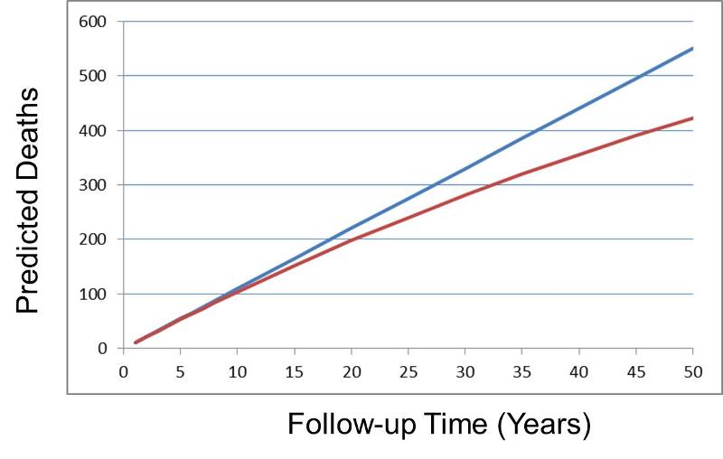
Nevertheless, note that the prediction from CI = IR x T gives quite reasonable estimates as long as the cumulative incidence remains less than 10% (equivalent to 100 deaths in the population of 1,000 in the above graph).