Analysis of Categorical Data
Up to this point we have discussed how to analyze continuous data. In this module we will address categorical data or count data. We will first describe one sample tests for a single proportion and then consider tests for association in cross tabulations.
After successfully completing this module, students will be able to:
Suppose we are interested in estimating the proportion of individuals in a population who have a certain trait. For instance, we might be interested in studying the proportion of children living near a lead smelter who have colic. The prevalence of colic in the general public is estimated to be as low as 7%. The data set "pbkiddat" contains information on a sample of children living near a lead smelter.
Rosner (Rosner, Fundamentals of Biostatistics, 1995) presents the data from an observational study which evaluated the effects of lead exposure on neurological and psychological function in children who lived near a lead smelter. Each child had his or her blood lead level measured twice, once in 1982 and again in 1983. These readings were used to quantify lead exposure. The control group (n=78) consisted of children whose blood lead levels were less than 40 ug/100mL in both 1982 and 1983, whereas the exposed group of children (n=46) had blood lead levels of at least 40 ug/100mL in either 1982 or 1983. We can use these data to make inferences on the general population of children living near a lead smelter.
Point estimate
We estimate the proportion, p, as:

where x is the number in the sample who have the trait or outcome of interest, and n is the size of the sample.
Hypothesis Tests
This hypothesis considers whether the population proportion is equivalent to some pre-specified value, p0. This value might be of historical interest or a result obtained in another study that we are trying to corroborate with our study data. A rule of thumb used to perform this test is that both np0 and n(1-p0) are greater than five.
To perform this test, we:

where n is the sample size.
Decision Rule:
Reject if Z > Zα/2, where Zα/2 is the 1-α/2 percentile of the standard normal distribution
Confidence Intervals
Additionally we can calculate confidence intervals for the sample proportion, again relying on the rule of thumb as stated above. The upper and lower limits of the confidence interval are given by:

Example
In the pbkid data set there were 124 children and 23 of them had colic.
We can first estimate the proportion of colicky infants as:

Using the information from the pbkid data set we can test if the prevalence of colic among children who live near lead smelter differs from that in the general public, which is around 7%.
Hypothesis:
Significance Level: 0.05
Test Statistic:

Decision Rule: Reject if |z| > 1.96.
Confidence interval:

Conclusion:
In our sample, the proportion of colic among children living near lead smelters was 0.19. We calculated a z-statistic of 5.24 which is greater than the critical value, 1.96 associated with a significance level α = 0.05. Thus we reject the null hypothesis and conclude that the prevalence of colic among children living near lead smelters is different from 0.07. The 95% confidence interval is 0.12 to 0.25.
Example
libname in 'C:\temp';
proc format;
value colicf 1="Yes" 2="No";
run;
data pbkid;set in.pbkid;
format colic colicf.;
run;
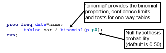
proc freq data=pbkid;
tables colic / binomial(p=0.07);
run;
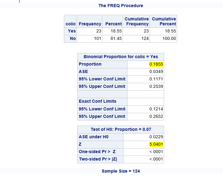
Notice that the Z statistic = 5.04 although our Z statistic was = 5.24. This is due to rounding.
The setup of the data is important. PROC FREQ will run a binomial test assuming that the probability of interest is the first level of the variable (in sorting order) in the TABLES statement. For example, the above statements run a binomial test on COLIC, which takes one of two numeric values – a 1 (Yes) or a 2 (No). The binomial test is applied to COLIC values of 1 because it is the first sorted value for that variable.
The LEVEL= option in the TABLES statement will modify the group level on which the test of proportions is performed. If the COLIC variable were set up to be 0=No and 1=Yes, a common format for categorical data, the default settings would result in a binomial test on the "No" values because 0 comes before 1 in sorting order. To make PROC FREQ run the binomial test on the "Yes" values of 1, use the LEVEL= option to look not at the first value of COLIC but the second as shown in the next example.
proc freq data=pbkid;
tables colic / binomial(p=0.05 level=2);
run;
If the variable COLIC were a character variable instead, the binomial test would, by default, consider the level of interest to be the first alphabetically, so if the responses are "no" and "yes," the level of interest would be "no". To have this switched, again use the LEVEL= option, specifying the character string "yes".
proc freq data=pbkid;
tables colic / binomial(p=0.05 level="Yes");
run;
You should always check the output to make sure you are reporting what you think you are reporting! Here, note the statement:
Binomial Proportion for colic = Yes
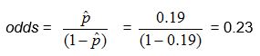
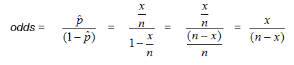
The odds of an event is simply the probability of the event occurring divided by the probability of the event not occurring.

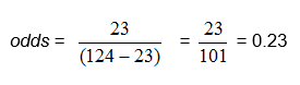
From the above example, in which there were 124 children and 23 of them had colic, we found
![]() , so
, so
Another way to think about the odds is the ratio of the number in the sample who have the trait or outcome of interest to the number who do not.
Substituting in for p, where x is the number in the sample who have the trait or outcome of interest, and n is the size of the sample,
In our example, we can compute the odds directly as the ratio of the number of babies with colic to the number with no colic:

Exercise: Complete the table below and calculate the odds in the table.
|
p |
1-p |
odds |
|---|---|---|
|
0.9 |
||
|
0.5 |
||
|
0.3 |
||
|
0.1 |
Note that if p is small, (1-p) is very close to 1, so the odds, p/(1-p), is a reasonable estimate of p.
Categorical variables may represent the development of a disease, an increase of disease severity, mortality, or any other variable that consists of two or more levels. To summarize the association between two categorical variables with R and C levels, we create cross-tabulations, or RxC tables ("Row"x"Column" or contingency tables), which summarize the observed frequencies of categorical outcomes among different groups of subjects. Here we will focus on 2 x 2 tables.
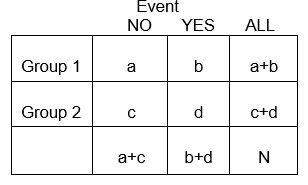
In general, 2 x 2 tables summarize the frequency of health-related (or other) events among different groups, as illustrated below in which Group 1 may represent patients who received a standard therapy, and Group 2 might be patients who received a new experimental therapy.
Example:
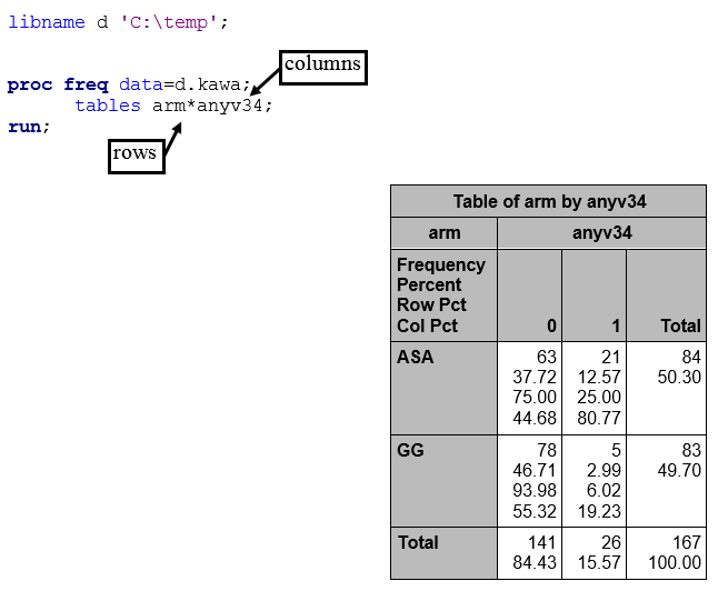
The primary outcome variable in the Kawasaki trials was development of coronary artery (CA) abnormalities, a dichotomous variable. One goal of the study was to compare the probabilities of developing CA abnormalities given treatment with Aspirin (ASA) or Gamma globulin (GG).
We might be interested in knowing whether the frequency of coronary artery abnormalities differed between these two groups, i.e., was one of these associated with fewer abnormalities. The answer to questions like this hinge on a comparison of the frequencies of these health events in the two treatment groups. Depending on the study design, one can compare either the probability of events or the odds of an event occurring.
Probability and Odds of Developing CA in Each of the Treatment Arms
The probability is computed as the number of "yes" values in each treatment category divided by the total number in the treatment category.
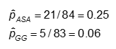
The odds is #Yes / #No. Here,
|
Always notice whether the outcome is in the rows or in the columns; it's very easy to mix these up! |
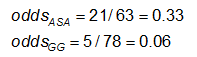
When we looked at the association between one binary variable and a continuous outcome, we summarized the association in terms of difference in means. What statistics are appropriate to represent the difference between two groups with respect to the probability of a binary event? There are at least three ways of summarizing the association:
Risk Difference RD = p1 - p2
Relative Risk (Risk Ratio) RR = p1 / p2
Odds Ratio OR = odds1/ odds2 = [p1/(1-p1)] / [p2/(1-p2)]
The study design determines which of these effect measures is appropriate. In a case/control study, the relative risk cannot be assessed, and the odds ratio (OR) is the appropriate measure. However, the OR will provide a good estimate of the relative risk for rare events (i.e., if p is small, typically 0.10 or smaller).
Cross-sectional studies assess the prevalence of health measures, so the odds ratio is appropraite. With prospective cohort studies either a rate ratio or a risk ratio is appropriate, although an odds ratio can also be calculated.,
For a more detailed review of effect measures, see the online epidemiology module on "Measures of Association."
Example: Using the previous data on CA abnormalities, the effect measures for those using ASA (aspirin) versus gamma globulin (GG) are as follows:
Exercise: Consider the measures of effect in the previous example. Why are the risk ratio and odds ratio so different (the RR suggests that, compared to the group treated only with ASA, the risk of coronary abnormalities is is 1/4 as high for those treated with GG; while the OR suggests the risk is 1/5 as high)?
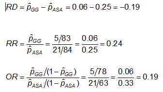
For a 2x2 table, the null hypothesis may equivalently be written in terms of the probabilities themselves, or the risk difference, the relative risk, or the odds ratio. In each case, the null hypothesis states that there is no difference between the two groups.
H0: p1 = p2
H1: p1 ≠ p2
H0: p1 - p2 = 0 (RD=0)
H1: RD ≠ 0
H0: p1/ p2 = 1 (RR=1)
H1: RR ≠ 1
H0: OR = 1
H1: OR ≠ 1
The difference in frequency of the outcome between the two groups can be assessed with the chi-squared test.

In each cell of the 2x2 table, O is the observed cell frequency and E is the expected cell frequency under the assumption that the null hypothesis is true. The sum is computed over the 2x2 = 4 cells in the table. As long as the expected frequency in each cell is at least five, the computed chi-square value has a χ2 distribution with 1 degrees of freedom (df).
Reject the null hypothesis if ![]() . For α = 0.05, the critical value is 3.84.
. For α = 0.05, the critical value is 3.84.
Example:
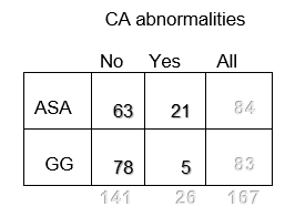
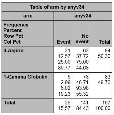
Observed frequencies
If there is no association between treatment and disease, the proportion of cases among those treated and not treated would be the same and would be equal to the proportion of cases in the entire study population.
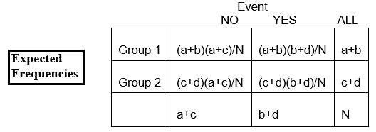
Expected frequencies:
Over all, among the 167 children, there are 26 with CA abnormalities and 141 without CA abnormalities. The proportion with CA abnormalities is 26/167, or 16%. If the null hypothesis is true, and the two treatment groups have the same probability of CA abnormalities, then we'd expect about 16% in each group to have CA abnormalities.
So, in the GG group of n=83, we'd expect 16% of 83 to have CA abnormalities. This is calculated as 0.16 x 83 = 13, and is called the expected frequency in that cell.
We can write this as
E11 = expected frequency in row 1, column 1
= expected number in group 1 who have the event (row 1, column 1)
And we calculate it as
E11 = (proportion we expect to have the event) x total number in (group) row 1
= [total number with the event (total of column 1 ) / total N] x number in (group) row 1
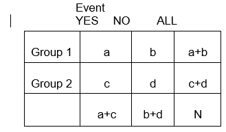
Using the notation in the table,
E11 = [(a+c)/N] x (a+b)
And we often rewrite this simply as
E11 = (a+b)(a+c)/N
In our example, let's calculate the expected frequency in the first cell ( E11) :
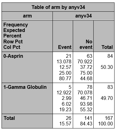
E11 = (83)(26)/167 = 12.92
We can calculate the expected frequencies in the other cells in the same way
The overall proportion without CA abnormalities is 141/167, or 84%. We expect about 84% of those in the ASA group to not have CA abnormalities, so the expected frequency in row 2, column 2, is E22 = 84% of 84, or 0.84 x 84, or approximately 71.
Using the table above, we could simply calculate it as
E22 = (c+d)(b+d)/N = (84)(141)/167 = 70.92
Exercise: How many of the children in the ASA group would you expect to have CA abnormalities if the null hypothesis is true? Try to work this out before looking at the answer below.
Note that the observed frequencies take on integer values, while the expected frequencies can take on decimal values.

We expect nearly 13 children in the GG group to have CA abnormalities, but only 5 actually did!
Notice that once we have calculated one expected frequency, the others can be obtained easily by subtraction! The number of degrees of freedom equals the number of cells whose expected frequency needs to be calculated; in a 2 x 2 table, this is 1.
Chi-Square test statistic

where O1,1 and E1,1 are the observed and expected counts in the cell in the first row and first column. For instance, O1,1 = a and E1,1 =(a+b)(a+c)/N. If the observed cell counts are different enough from the expected, then we cannot conclude that the two probabilities are equal.

H0: The odds of CA abnormalities are the same across treatment groups (OR=1)
H1: The odds of CA abnormalities are not the same across treatment groups (OR≠1)
The significance level is 0.05.
The test statistic is calculated to be 11.43. Since our test statistic is greater than 3.84 (the chi-square critical value for 1 degree of freedom), we reject the null hypothesis and conclude that the odds of CA abnormalities are not the same in the two treatment groups.
Example:
The Kawasaki study data are in a SAS data set with 167 observations (one for each child) and three variables, an ID number, treatment arm (GG or ASA), and an indicator variable for any CA abnormality at visit 3 or visit 4.
The PROC FREQ statement has an option that defines the order in which values appear in frequencies and crosstabs generated by PROC FREQ.
The default is ORDER=INTERNAL, which means that data is ordered (alphabetically or numerically) by the unformatted values of the data. For example, the ARM variable in the above example takes on a value of 'ASA' or 'GG,' and thus, by default, the ASA values will appear before the GG values in the PROC FREQ output.
The option ORDER=FORMATTED will order the data by (ascending) formatted values of variables. The impacts of other ORDER= options are given at the end of this module.
Formatting the outcome so that the event is in the first column
Using the format below, since "E" comes before "N" alphabetically, "Event" will be in column 1 and "No event" in column 2. However, ASA will be in row 1 since ASA is formatted "0-Aspirin" and GG is formatted "1-Gamma Globulin".
proc format;
value $armf "ASA"="0-Aspirin" "GG"="1-Gamma Globulin";
value eventf 0='No event' 1='Event';
run;
proc freq data=d.kawa; order=formatted;
format arm $armf. anyv34 eventf.;
tables arm*anyv34;
run;
Other Options
We can keep including a format statement in each proc but let's instead format them in a data step.
data one;set d.kawa;
format arm $armf. anyv34 eventf.;
There are several options that can be included after a / in the TABLE statement.
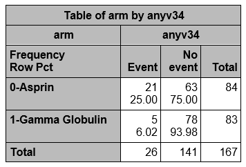
proc freq data=one order=formatted;
tables arm*anyv34 / nocol nopercent;
run;
proc freq data=one order=formatted;
tables arm*anyv34 / expected ;
run;
proc freq data=one order=formatted;
tables arm*anyv34 / chisq ;
run;
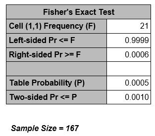
The 2 x 2 table is produced as above, plus the following output.
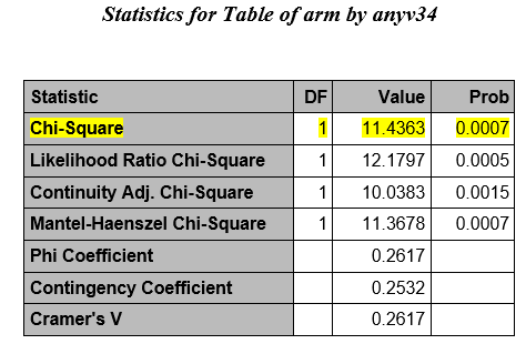
The highlighted row contains the chi square statistic and its associated p-value
|
Note: If > 20% of the cell frequencies are <5, SAS will print a warning, and you should not use the chi-square test. Instead, use the Two-sided Fisher's Exact Test (printed by default when the table is 2 x 2). |
proc freq data=one order=formatted;
tables arm*anyv34 / measures;
run;
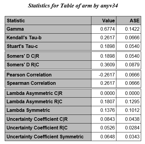
The above measures can be ignored for now; we will focus on the following measures, the odds ratio and the relative risk (column 1) which considers column 1 to contain the event of interest.
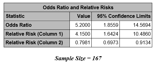
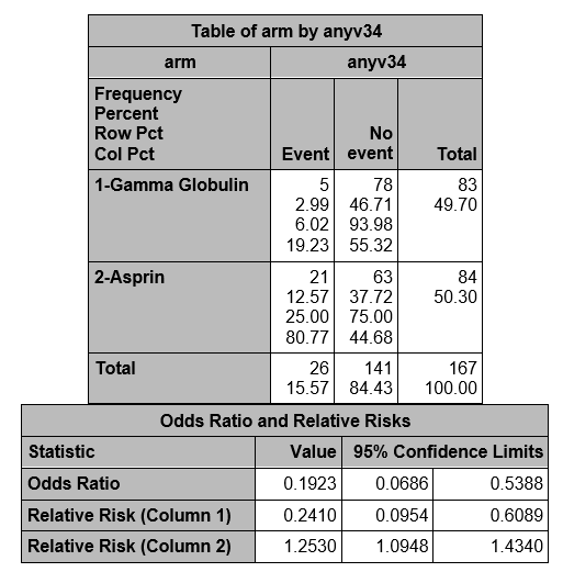
Recall that we obtained the following effect measures, comparing those on GG to those on ASA alone:
Estimated effect measures (GG vs. ASA):
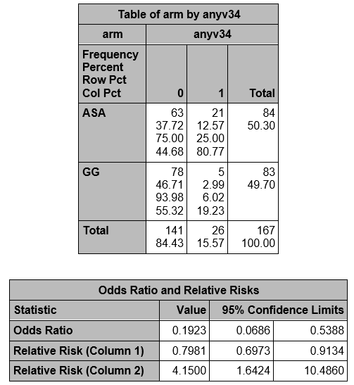
Note that the RR produced by proc freq is RR = 4.15 - because they are comparing ASA to GG! The comparison is always the first row as compared to the second row. Here, ASA is in row 1 since ASA is formatted "0-Aspirin" and GG is formatted "1-Gamma Globulin". Similarly, the OR is the ratio of the odds of CA abnormalities in the ASA arm compared to the GG arm, instead of GG compared to ASA.
|
SAS calculates the odds ratio assuming that column 1 is the event of interest and row 1 is the treatment group of interest (meaning that column 2 is the reference event and row 2 is the reference treatment group). It calculates the relative risks also assuming row 2 is the reference group. It is preferable to arrange the data to make the outcome of interest appear in the first column and the target group to appear in the first row and to use formatting if it is not. If the data are not in this format, the odds ratio and relative risks are computed but the interpretation may be different than what is intended. |
We should re-format to ensure that we are comparing the new treatment, GG, to the usual treatment, ASA.
proc format;
value $armf "ASA"="2-Aspirin" "GG"="1-Gamma Globulin";
value eventf 0='No event' 1='Event';
run;
proc freq data=two order=formatted;
tables arm*anyv34 / measures;
run;
Now the measures compare GG to ASA, and we see the same measures we obtained by hand.
Table options can be combined in the TABLE statement; the following statement would provide observed and expected frequencies, row percentages, effect measures and the chi square
proc freq data=two order=formatted;
tables arm*anyv34 / chisq expected measures nocol nopercent;
run;
Technical Summary
H0: The odds of a CA abnormality in the GG group is the same as in the ASA group (OR = 1).
H1: The odds of a CA abnormality in the GG group is not the same as in the ASA group (OR ≠ 1).
Level of significance: 0.05
Estimates of interest:
![]()
Conclusion:
Reject H0. There is significant evidence (at α=0.05) that the OR is not equal to 1 (p-value < 0.001). The estimated OR = 0.19 (95% CI= 0.0686, 0.5388) with the odds for developing CA abnormalities in the GG group being 0.19 times the odds for developing CA abnormalities in the ASA group.
Write-up
Methods
A chi-square test was performed to compare the probability of coronary artery abnormalities in patients with Kawasaki disease receiving gamma globulin treatment compared to those receiving aspirin treatment. We employed a 0.05 significance level for this test.
Results
We calculated an odds ratio of 0.19 with a 95% confidence interval of 0.0686-0.5388. With a p-value of 0.0007 we reject the null hypothesis and conclude that the odds of a CA abnormality in the GG group is not the same as the ASA group.
proc freq data=one;
tables arm*anyv34 / measures;
run;
Exercise: See if you can arrive at, and interpret, the estimates in the above table.
If an observation has any variable missing, the default is to exclude it from the table and all calculations. You can override this by using the missing option.
Example:
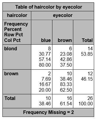
Suppose you have a data set with 28 observations on hair color (brown or blond) and eye color (blue or brown), but one person is missing hair color and another is missing eye color.
data one;
input haircolor $ eyecolor $;
cards;
brown blue
.
.
blond blue
;
proc freq;tables haircolor*eyecolor;run;
|
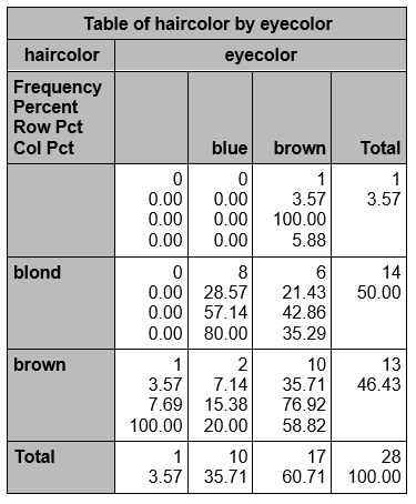
Using the missing option will display "missing" as a level of the variable. Those observations will count in totals and percentages. |
proc freq;tables haircolor*eyecolor/missing;run;
NOTE: All of the analyses shown above assume that data are in a file with one observation per person. To instead perform an analysis with data from an existing table input the observed cell frequencies and use a weight statement with the weight equal to the cell frequency.
Example (Kawasaki data)
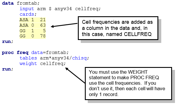
This will produce the same output as we found above.
Chi-square tests can also be used for for R x C tables
H0: the two categorical variables are independent.
H1: the two categorical variables are not independent
The chi squared test can be used just as above, with the expected frequencies calculated in a similar fashion.

where the sum is computed over the RxC cells in the table. As long as no more than 20% of the cells have expected frequencies < 5, the computed chi-square value may be compared to the critical chi-square value with (R-1)(C-1) degrees of freedom (df) and a pre-specified level of significance (α).
Reject if ![]()
Example:
Suppose you have a data set in which people are classified by hair and eye color but with three hair colors and two eye colors. You test
H0: Hair and eye color are independent.
H1: Hair and eye color are not independent
data one;
input haircolor $ eyecolor $;
cards;
brown blue
.
blond blue
;
proc freq;tables haircolor*eyecolor/chisq;run;
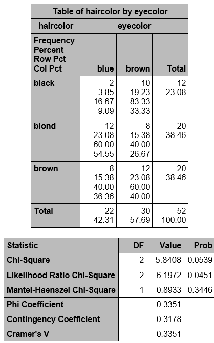
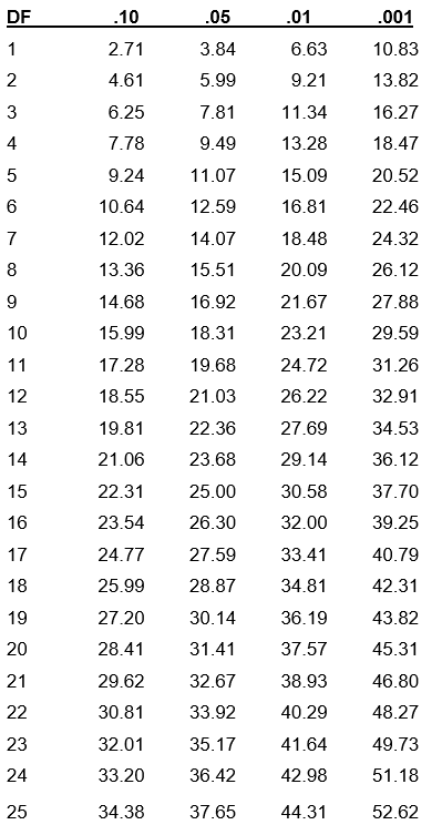
Notice that df = (3-1)x(2-1) = 2. We did not explicitly check the expected frequencies, but SAS did not warn us that they were not sufficient, so we can use the test. Using the table at the end of this lecture, we see the critical value of χ2 with 2 degrees of freedom, and α = 0.05 is 5.99. The χ2 statistic = 5.8408 which is just less than the critical value, so we do not reject Ho. Alternatively, we can compare p to α = 0.05. Here, p = 0.0539, which >0.05 and we do not reject Ho. We conclude that we do not have enough evidence to say that hair and eye color are not independent.
Example:
Suppose you have yet another data set in which people are classified by hair and eye color but with three levels of hair color and three levels of eye color.
proc freq;tables haircolor*eyecolor/chisq expected nocol nopercent;run;
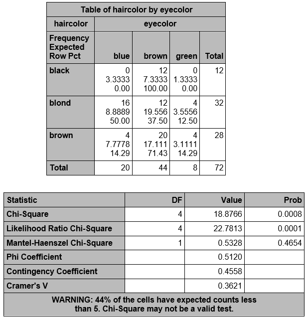
Here we are warned that the chi square test may not be valid, because 44% of the expected counts are < 5. Notice that 5 of the 9 cells (55%) have observed counts <5, but that is not relevant.
One option is to combine levels. Here we can combine black and brown hair or we can combine blue and green eyes. Let's combine levels of eye color.
data two;set one;
length new_eyecolor $ 10;
new_eyecolor=eyecolor;
if eyecolor in ('blue','green') then new_eyecolor='blu-grn';
proc freq;tables haircolor*new_eyecolor/chisq;run;
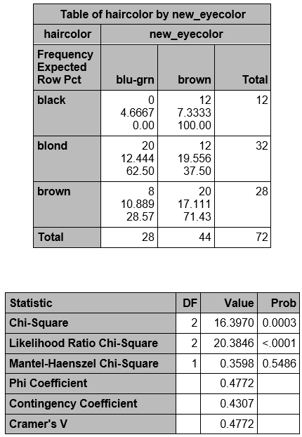
Now, there is only 1 of 6 (16%) cells with expected frequency <5, so the chi square test is valid.
df = (3-1)x(2-1) = 2. The χ2 statistic = 16.3970 and p = 0.0003, so we do reject Ho and conclude that we have evidence that hair and eye color are not independent.
the magnitude of the differences between the two groups using effect measures and confidence intervals for those measures. We can calculate these effect measures and their confidence intervals when the data come from a 2x2 table in the following manner.
![]()
We can calculate the confidence interval for this quantity as:


The confidence interval can be calculated by taking the log of the relative risk and assuming that is normally distributed. So the confidence interval for the log of the relative risk is given by:

Therefore the estimated confidence interval of the relative risk is:


The confidence interval for this quantity is again estimated using a log transformation on the OR and assuming normality of that quantity. Therefore the confidence interval for the log of the odds ratio is:

where a, b, c, d are the numbers of observations in each of the four cells of a 2x2 table. The confidence interval for the odds ratio can then be calculated as:
Let's go back to the data comparing the frequency of coronary artery abnormalities between subjects treated with gamma globulin (GG) versus aspirin (ASA) and compute the confidence intervals for these three measures of effect (measures of association).
Risk Difference: RD = -0.19
The 95% confidence interval for the RD is estimated as:

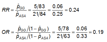
Relative Risk: RR = 0.24
The 95% confidence interval for the log of the relative risk is estimated:

So that the confidence interval of the relative risk is:
![]()
Odds Ratio: OR = 0.19
The 95% confidence interval for the log of the odds ratio is:

.Therefore, the confidence interval for the odds ratio is obtained by exponentiation these values:
All of these estimates and their corresponding confidence intervals indicate that those with ASA have a statistically significant higher risk (or odds) of CA abnormalities than those with GG.
The PROC FREQ statement has an option that defines the order in which values appear in frequencies and crosstabs generated by PROC FREQ. The default is ORDER=INTERNAL, which means that data is ordered (alphabetically or numerically) by the unformatted values of the data. For example, the ARM variable in the above example takes on a value of 'ASA' or 'GG' and thus by default the ASA values will appear before the GG values in the PROC FREQ output. The impact of other ORDER= options are given in the table below.
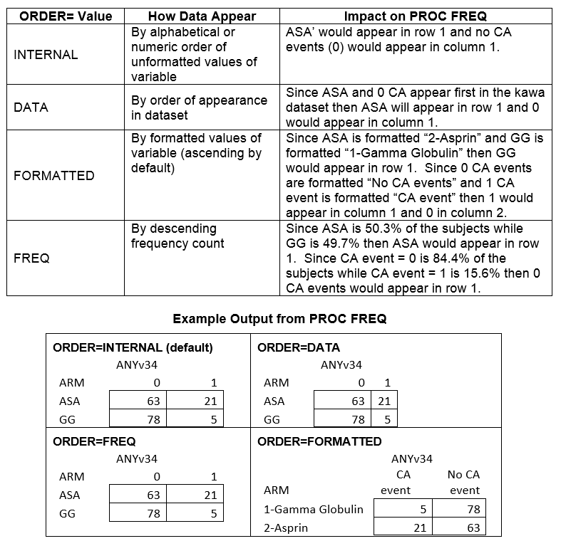
Which should you use? In general, it's worth arranging the PROC FREQ output so that the outcome of interest appears in the first column and the target group appears in the first row. In the example above, the output table should be arranged so that ARM = 'GG' is in the first row and ANYv34=1 is in the first column.
AREA ABOVE CUTOFF (CRITICAL VALUES FOR SPECIFIED ALPHA)