

Two-Sample Test of Means
In the previous module, we discussed the one sample t-test, which compares the mean of one sample to a predetermined constant, and the paired t-test, which compares the mean difference between two variables in a single sample. Now we wish to compare two independent groups with respect to the mean of an analysis variable. In the cholesterol example, we might wish to compare the average age of subjects who had coronary events by 1962 to the average age of subjects who did not have a coronary event by 1962.
Assumptions:
- Independent observations.
- The two groups are independent.
- The two populations from which the data are sampled are each normally distributed.
Hypothesis:
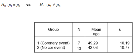
H0: μ1=μ2 vs. H1: μ1 ≠ μ2
Point Estimate:
![]() is the point estimator of .
is the point estimator of .![]()
Confidence Interval:
![]()
Test statistic:

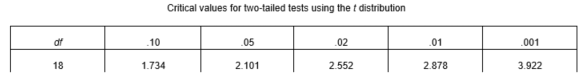
As with the one-sample t-test, the t-statistic calculated using the above formula is compared to the critical value of t (which can be found in the t table using the df and a pre-specified level of significance, α). Again, if the absolute value of the calculated t-statistic is larger than the absolute value of the critical value of t, the null hypothesis is rejected.
Estimating the Standard Error of the Difference Between Means
There are two formulas used to estimate the standard error of the difference in means, ![]() . One is appropriate if the population variances are equal, and the other is to be used if we cannot assume that they are equal.
. One is appropriate if the population variances are equal, and the other is to be used if we cannot assume that they are equal.
Test for Equality of the Variances
To determine which of the two formulas to use, we first test the null hypothesis that the population variances of the two groups are equal.
First, test H0: σ12= σ22
The test for equality of variances is based on the distribution of the ratio of the variances and uses the F statistic, F = s12/s22. This statistic has a distribution in the F-family of distributions and is indexed by two numbers: the denominator degrees of freedom and the numerator degrees of freedom. The degrees of freedom for the test above are (n1-1) for the numerator and (n2-1) for the denominator; thus the values of the test statistics should be compared to the critical value of the F distribution with (n1-1) and (n2-1) degrees of freedom.
Note that the F distribution is not symmetric (as are the normal and t distributions), which makes it more difficult to look up the critical values. For example, the area above z=1.96 is 0.025, as is the area below z=-1.96. So, if α=0.05, the critical values of z are ±1.96. The table thus only needs to show one side of the distribution. The F distribution is not as simple. For example, with (12,6) degrees of freedom, the area above 5.37 is 0.025, and the area below 0.268 is 0.025. So we would reject a test if F is < 0.268 or > 5.37. Notice that if F<1, we compare F to the lower critical value, and, if F>1, we compare F to the upper critical value.
The trick is to note that if we compare the larger variance to the smaller, so that F = (larger variance)/(smaller variance), the F statistic will be always be >1. Since F>1,we will use the upper critical value.
- Choose the larger estimated variance to be the numerator and the smaller estimated variance to be the denominator. For this example we will assume that s1 is larger than s2 and compute , F = s12/s22.
- Compare F to the upper critical value (corresponding to α/2) of the F distribution. If F is greater than the critical value for a given level of significance, the null hypothesis is rejected and we can conclude that there is significant evidence that the two population variances are not equal.
Example (from Dixon and Massey):
We would like to compare the average age of subjects who had coronary events by 1962 to the average age of subjects who did not have a coronary event by 1962.
Step 1: Check the assumption of equal population variances ( ![]() ).
).
We use the No coronary event group as the numerator since it is larger. Then the degrees of freedom are (13-1) and (7-1), usually written as (12,6).
The critical value of the F test (if α=0.05, we use the upper critical value, with 0.025 above it) is
![]()
We will rely on SAS to perform this test and will not expect you to look up these critical values.
Calculate the F statistic,
![]()
F < the critical value so we do not reject the null hypothesis that the variances are equal and thus can use the pooled standard error.
Note, the F test is sensitive to departures from normality and may have low power to detect differences in the variances. Thus, its usefulness as a preliminary test of equality of variances is limited. It is helpful to examine the variability in the two groups by comparing the sample variances and looking at boxplots to help decide which standard error assumption is appropriate.
proc boxplot
proc boxplot provides boxplots for a continuous variable var by a grouping variable, group. Note: this requires that the data are sorted by the grouping variable.
proc boxplot data=dix;
plot var*group / cboxes=black;
run;
Let's inspect the boxplots in each of the two groups (cor=1 and cor=2)
/* Sort the data so we can look at separate proc Boxplots */
proc sort data=dixonmassey;
by cor;
run;
/* Good way to summarize the data and visually check homoscedasticity assumption*/
title 'Box Plots of Age By Coronary Event';
proc boxplot data=dix;
plot age*cor / cboxes=black;
run;
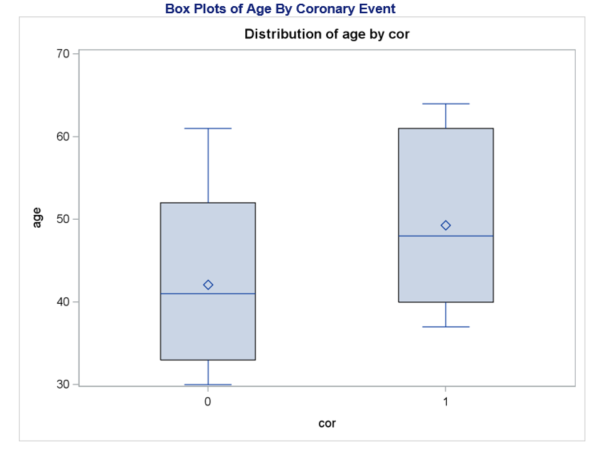

Do you think the variances look equal?
Estimating the Standard Error of the Difference Between Means
Assuming equal population variances (σ12= σ22)
If σ12= σ22, the pooled variance, Sp, may be used to estimate the common variance, σ2.

and the standard error of the difference in means is estimated as

The degrees of freedom for the t-test in this case are n1+n2-2.
Not assuming equal population variances (not assuming ![]() )
)
If we cannot assume ![]() , the standard error of the difference in means is estimated as:
, the standard error of the difference in means is estimated as:

Calculating the degrees of freedom in this situation is complicated (see Statistical Methods, 8th edition, by GW Snedecor and WG Cochran, page 97). In our hand calculations we will use the minimum of (n1-1) and (n2-1) to approximate the degrees of freedom for the above t-test; when using SAS the correct number of degrees of freedom will be calculated and used.
In our example, we did not reject the hypothesis of equal variances, so we pool the variances in calculating the standard error.
Step 2: Calculate the standard error of the difference in means
![]()

df= n1+n2-2 = 18.
Step 3: Calculate the t statistic to test ![]()

The critical value of t with 18 df and α=0.05 is ± 2.101.
Conclusion
The mean age of the group with coronary events was 49.29 (N = 7, SD = 10.19) compared to a mean age of 42.08 (N = 13, SD = 10.77) for the group without coronary events. Since the t statistic with 18 df of 1.45 does not lie outside the critical values of ± 2.101 for α =0.05, we fail to reject the null hypothesis that the mean age is the same in the group of subjects with coronary events and the group of subjects without coronary events. We cannot conclude that the average age is statistically different for those who had coronary events compared to those who did not.