
Introduction to SAS for Windows and Review of Basic Statistics
About the Course
This course introduces statistical computing using Statistical Analysis Systems (SAS). The emphasis is on manipulating data sets and basic statistical procedures such as t-tests, chi-square tests, correlation, and regression. SAS is a statistical package and a programming language. As with any language quite a bit of practice is required in order to be fluent.
Why take this course?
Statistics with SAS
Statistical knowledge is crucial to understand and interpret SAS output. Although several statistical concepts and methods will be reviewed, this course assumes that you have completed an introductory course in biostatistics or in statistics. Please see the instructor if you have not fulfilled this requirement.
After completing this modules, the student will be able to:
At the end of this module there is also a brief review of basic biostatistics.
In this class, we will use SAS version 9.3. This version should already be installed on your lab computers. If you have SAS version 9.4 installed on your computer, that's fine. If you happen to have an earlier version installed on your computer, please see your instructor
From the Windows Desktop, select the Start menu, the Programs menu, the SAS menu, and finally SAS 9.3 (English).
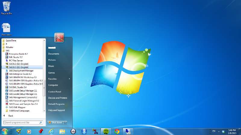
NOTE: The appearance of your computer screen will differ depending on which version of Windows you are using.
Once SAS has started, the screen will look similar to the following:
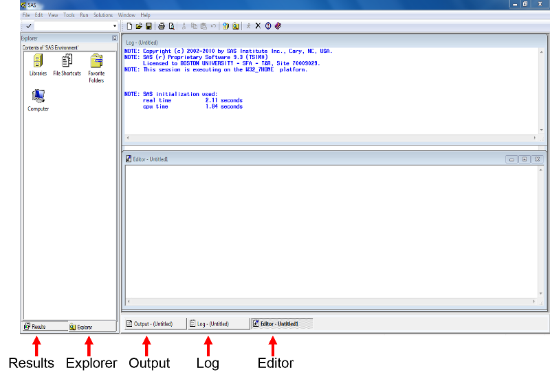
The main SAS window is divided into several sub-windows: the menu and toolbar along the top of the window, the explorer/results browser along the left hand side, the log to the top right, the program editor below the log on the bottom right, and the windows bar along the bottom.
The Editor (Program Editor) window is a text editor that facilitates writing SAS programs (code). The Log window displays system messages, errors, and resource usage and is thus used to review program statements. The Output window displays output from statistical procedures run within the SAS program; however this is no longer the default. In SAS 9.3 output is sent to the Results Viewer which opens automatically when you run a procedure that generates output. The Results window displays a map of the Output window, and is useful for navigating the results of complicated analyses. Finally, the Explorer window contains all of the data sets in the current SAS session.
These windows can be moved or resized as desired. Only one SAS window is active at a time. The active window will have a shaded title bar at the top of the window, and a highlighted windows bar at the bottom of the screen. In the above example, the Program Editor is the active window, with an "Untitled" program name. Note that the menu options for the SAS toolbar along the top of the screen depend on which window is currently active.
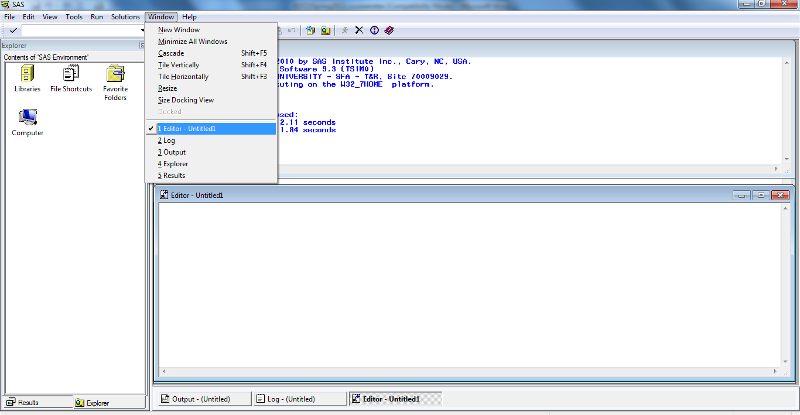
The active window can be changed by clicking on that window with the mouse, or by selecting the desired window from the Window menu.
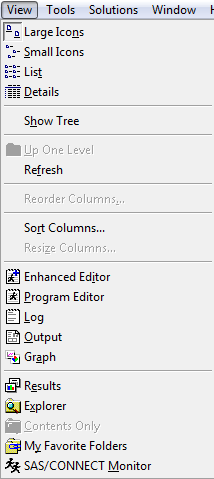
The active window can also be changed using the View menu.
We will now consider a simple program, which creates a SAS data set using a SAS data step (DATA) and calculates simple descriptive statistics (sample size, mean, and standard deviation) using a SAS procedure (PROC). A SAS data step is primarily used to create and modify data sets, and a SAS procedure is primarily used to analyze data. We will review these concepts more in a bit.
All data used by SAS is stored in a data set.
|
A data set is a matrix (or box) that contains a column for every variable and a line for each observation (e.g., subject). Data sets can be entered in the SAS programming code or can be read in from a variety of external sources, such as text files, and Microsoft Excel. In subsequent classes we will discuss reading in data sets from external files. Once a data set has been created, commands or procedures can operate on these data sets. |
Many procedures are implemented in SAS. Their scope varies; some examples are:
The name of the procedure is often suggestive of the scope of that procedure.
We will begin by typing the following commands into the Program Editor:
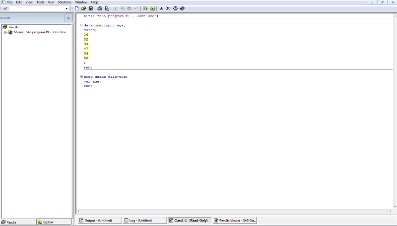
Line 1: defines a title that will appear on each page of output. Title statements are optional, but they help provide information about the program and are a useful addition to most analyses. In this class, we will often require title statements for assignments.
Line 2: is blank.
Line 3: creates a data set named one.
Line 4: creates two variables named age and gender.
Line 5: indicates to SAS that data will follow. Instead of cards; the code datalines; may also be used to tell SAS to expect data on the next several lines. SAS expects to see data until the next semi-colon, which is on line 12 in this programming code.
Lines 6-11: provide 6 observations of age and gender in this data set
Line 12: the semi-colon indicates to SAS that there are no further data set observations.
Line 13: indicates the end of the data step.
Line 14: is blank.
Line 15: tells SAS to use the means procedure on the data set named one.
Line 16: tells SAS to run the means procedure on the variable age.
Line 17: indicates the end of the means procedure.
|
|
Note that the program has not yet been executed!
To execute (run) the program first make sure the Editor is active by clicking on the Editor window, and then either
select the Submit option from the Run menu,
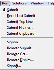
or click the "Run" button of the "little person running" ![]() located on the toolbar at the top of the screen.
located on the toolbar at the top of the screen.
You can also run just part of a program by selecting the part that you want to run and then using the Submit command from the Run menu or by clicking on the "Run" icon
Once the program has been run, a log of commands will appear in the Log window and, as long as there are no errors in the programming code, the output will appear in either the Output window and/or in a new window named Results Viewer. Note that the new log information and output are appended to the bottom of the Log window and Output or Results Viewer windows respectively. To view the log window, select the log tab from the bottom toolbar.
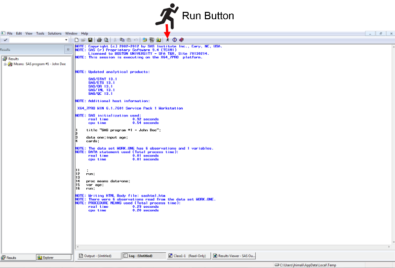
The first 4 lines of the log are produced when SAS is first opened. The following lines are added when the program editor is run. If there was a problem with the code, Errors and/or Warnings would be seen in the log. Errors messages are posted in red font and warnings in green font. A warning does not necessarily mean that there is an error in the program, however the warnings should be read carefully.
SAS indicates that data set WORK.ONE was created and includes one variable with 6 observations.
The WORK prefix for data set ONE indicates the SAS library name where SAS stores the data set. The WORK library is temporary and thus data sets stored here only exist as long as the current SAS session is open and will be deleted when SAS is closed. The topic of SAS libraries will be covered in more detailed in module 2.
|
After running the program code, ALWAYS check the log file for errors. Programmers of all levels make mistakes. However, expert programmers find and correct their mistakes quickly. Checking and understanding the statements in the log file is essential to proficient programming.
|
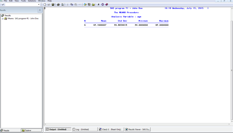
By default the output from your program, in this case your title and means, will appear in HTML format in the results viewer window.

This is different than previous versions of SAS, where the program output was sent as a text listing to the output window by default.
In some cases the formatted HTML output may be preferred as it is easier to read, but in other circumstances the text based listing format may be easier to work with. Fortunately the SAS output defaults can be easily changed to provide both.
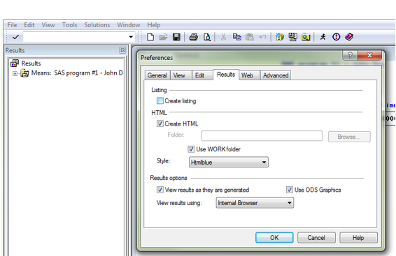
This is done by selecting Tools![]() Options
Options![]() Preferences from the menu at the top of the main SAS window and opening the Results tab (mnemonic TOPR). The following display shows the SAS Results tab with the default settings set to create only HTML output. Check the Create listing box to obtain both types of results.
Preferences from the menu at the top of the main SAS window and opening the Results tab (mnemonic TOPR). The following display shows the SAS Results tab with the default settings set to create only HTML output. Check the Create listing box to obtain both types of results.
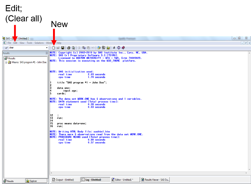
To clear the log or output window make sure the window is active and then either type "clear" in the Command box, or click on the blank page button on the left side of the toolbar, or select the Clear All option from the Edit menu. Note that the Editor window can also be cleared this way. If the Editor window is mistakenly cleared, immediately press Ctrl Z or select the Undo option from the Edit menu to undo the clear. The Results Viewer cannot be cleared in this manner; we will tell you how to clear the Results Viewer in Class 2.
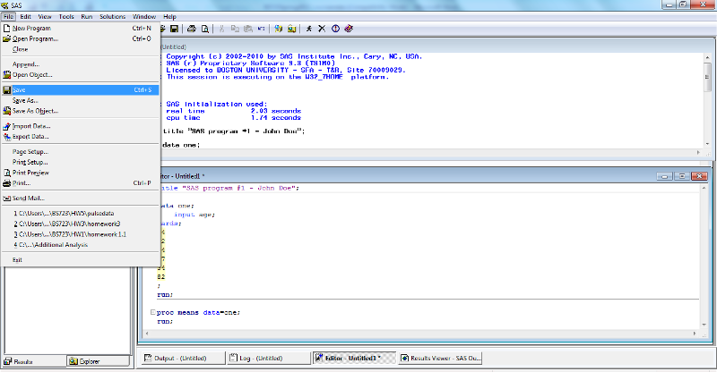
The program should be saved regularly. To save, select the Editor window to make it active; then select the Save option from the File menu. (You can also press CTRL+S)
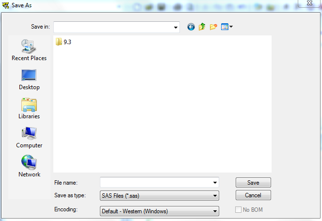
Like the program editor, the contents of the results viewer, output and log windows can also be saved. To save the results viewer, output or log click on the tab to make the file active and then select the Save option from the File menu. The file extensions for the log is '.log'. The file extensions for the output is '.lst'.The file extensions for the results viewer is '.mht'.
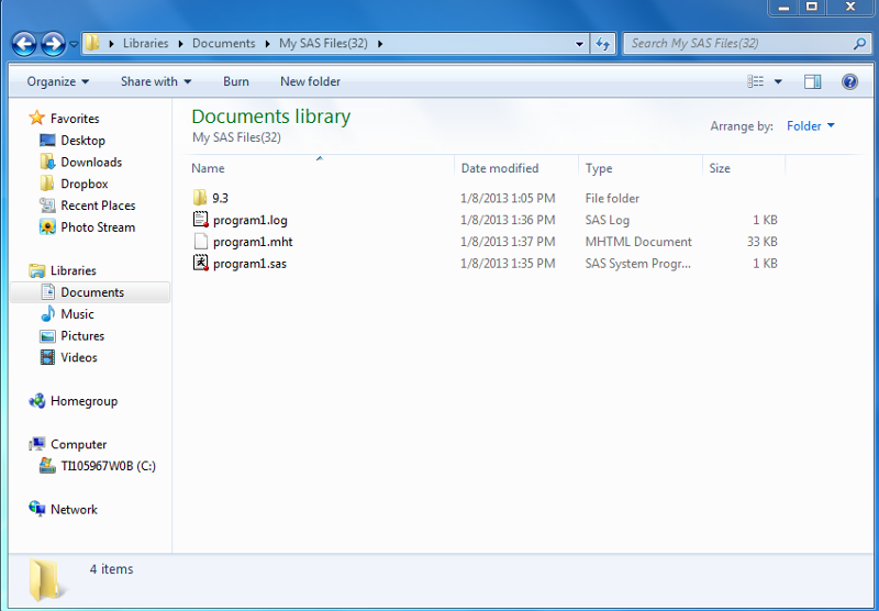
In the example below there are 3 files: program1.mht (HTML results), program1.log (log file), and program1.sas (SAS program editor). Like any saved files, these files can be copied to a USB drive or e-mailed as an attachment for safekeeping. The .sas, .log and .lst files may also be opened and edited within a word processor such as WordPad or notepad. The .mht files will open in a web browser.
To leave SAS, select Exit from the File menu.
Successful completion of a formal course in biostatistics or statistics is a prerequisite for this class, but review of the following online learning modules may be very beneficial.
Please take the time to review basic biostatistics concepts and see the instructor if you have not fulfilled this prerequisite.
Below are a few examples of descriptive statistics. These will be covered in more depth throughout the rest of the course.
Continuous Variables
Measures of Central Tendency
Measures of Dispersion
Graphs
Categorical Variables
Descriptives
Graphs
Continuous and Categorical
Two Continuous Variables
Two Categorical Variables
Note, in addition to categorical and continuous variables, there are identifier variables such as ID or Name. Usually, descriptive statistics should not be calculated for identifier variables.
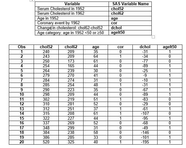
Note: The 'dixonmassey' data set is from Dixon WJ and Massey F Jr., Introduction to Statistical Analysis,, Fourth Edition, McGraw Hill Book Company, 1983.
Sample Size = 20 males
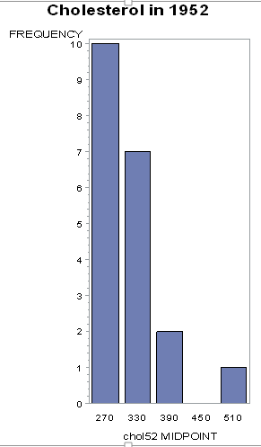
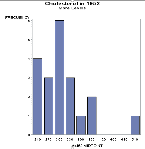
Graphical Summaries - Continuous Variables
Example: chol52
Median:

Mean:


Range:
![]()
Lower Quartile:

Upper Quartile:

Interquartile Range:
![]()
Variance:


Standard Deviation:
![]()
Counting: 7 subjects had a coronary event by 1962.
Proportions: 7/20 = 35% of patients had a coronary event by 1962.
Mean of Chol52
For cor = 0, 301.85
For cor = 1, 328.43
Correlation: r = -0.11
Regression: Chol52 = 341 – 0.66*age.
cor and Agelt50

