Categorical Data Analysis

Table of Contents»

Contributing Authors:

Ching-Ti Liu, PhD, Associate Professor, Biostatistics

Jacqueline Milton, PhD, Clinical Assistant Professor, Biostatistics

Avery McIntosh, doctoral candidate

This module will enable you to conduct analyses of tabular or categorical data in R.

Specific topics will include: 

1. Single proportion
2. Two independent proportions
3. k proportions

Learning Objectives

By the end of this session students will be able to:

1. Explain key procedures for the analysis of categorical data
2. Use R to perform tests on proportions for one, two or k categorical variables
3. Interpret the results of tests on proportions for one, two or k categorical variables

Analysis of Categorical Data

For a continuous variable such as weight or height, the single representative number for the population or sample is the mean or median. For dichotomous data (0/1, yes/no, diseased/disease-free), and even for multinomial data—the outcome could be, for example, one of four disease stages—the representative number is the proportion, or percentage of one type of the outcome.

For example, 'prevalence' is the proportion of the population with the disease of interest. Case-fatality is the proportion of deaths among the people with the disease. The other related term is 'probability'. For dichotomous variables the proportion is used as the estimated probability of the event. In epidemiology, comparison of two proportions is more common than two means. This is mainly because a clinical or public health decision is often based on a dichotomous outcome and less on the level of difference of the mean values.

Exploratory Analysis with Tabular/Categorical Data

As we saw in the second module in this series, categorical data are often described in the form of tables. We used a number of commands to create tables of frequencies and relative frequencies for our data. Suppose we use the airqualityfull.csv dataset, which recorded daily readings of airquality values.

 First read in the data:

> aqnew <- read.csv("airquality.new.csv",header=TRUE, sep=",")

Do you recall what the following commands do? Let's do a little review:

> table(goodtemp)

> table(goodtemp,badozone)

> table(goodtemp,badozone,Month)

> ftable(goodtemp+badozone~Month)

> table.goodbad<-table(goodtemp, badozone)

> margin.table(table.goodbad,2)  # here x is a matrix/data frame

> prop.table(table.goodbad,1)    # here y is a matrix/data frame

> barplot(table.goodbad, beside=T, col="white", names.arg=c("high ozone","low ozone"))

Choosing the Best Type of Plot

With all the available ways to plot data with different commands in R, it is important to think about the best way to convey important aspects of the data clearly to the audience. Some situations to think about:

A) Single Categorical Variable

Use a dot plot or horizontal bar chart to show the proportion corresponding to each category. The total sample size and number of missing values should be displayed somewhere on the page. If there are many categories and they are not naturally ordered, you may want to order them by the relative frequency to help the reader estimate values.

#single variable

goodtemp.1<-ifelse(goodtemp=="low", 0, 1)

barplot(table(goodtemp.1), col=c("lightblue","darkred"),main="Low (0) vs. High (1) Temp",ylab="Count")

#...or horizontal:

barplot(table(goodtemp.1), col=c("lightblue","darkred"),main="Low (0) vs. High (1) Temp",ylab="Count",horiz=T)

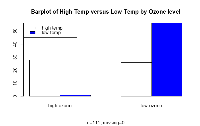
B) Categorical Response Variable vs. Categorical Independent Variable

This is essentially a frequency table, which can be depicted graphically (e.g., barplot)

#categorical response vs. categorical predictor

barplot(table.goodbad,beside=T,col=c("white","blue"), names.arg=c("high ozone","low ozone"), main="Barplot of High Temp versus Low Temp by Ozone level", sub="n=111, missing=0")     

legend("topleft", legend=c("high temp", "low temp"),fill=c("white", "blue"))

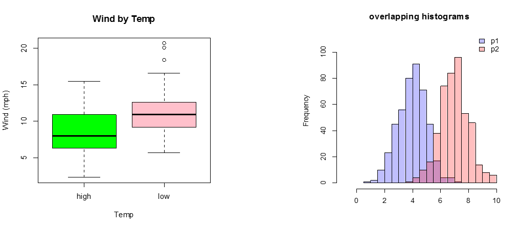
C) Continuous Response Variable vs. Categorical Independent Variable

If there are only two or three categories, consider box plots. Occasionally, a back-to-back histogram can be effective for two groups.

boxplot(Wind~goodtemp, xlab="Temp", ylab="Wind (mph)", main="Wind by Temp",col=c("green","pink"))

p1 <- hist(rnorm(450,4))                     # centered at 4

p2 <- hist(rnorm(450,7))                     # centered at 7

plot( p1, col=rgb(0,0,1,1/4), xlim=c(-1,10),ylim=c(0,110),xlab="",main="overlapping histograms")

plot( p2, col=rgb(1,0,0,1/4), xlim=c(-1,10),ylim=c(0,110), add=T)

legend('topright',c('p1','p2'),fill = c(rgb(0,0,1,1/4),rgb(1,0,0,1/4)), bty = 'n')

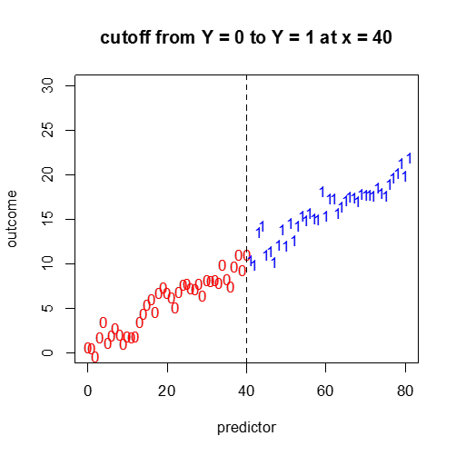
D) Categorical Response vs. a Continuous Independent Variable

Not so easy. A continuous plot with cutoff points? We will cover this more in the next module.

#continuous predictor, binary outcome...?

x1<-seq(0,40,1)

x2<-seq(41,81,1)

for(i in 1:41){

y1[i]<-(1/5)*x1[i]^(1/10)+(1/4)*x1[i]+rnorm(1,0,1)

y2[i]<-(1/5)*x2[i]^(1/10)+(1/4)*x2[i]+rnorm(1,0,1)

}

plot(x1,y1,pch="0",main="cutoff from Y = 0 to Y = 1 at x = 40",col="red",ylim=c(0,30),xlim=c(0,80),xlab="predictor",ylab="outcome")

points(x2,y2,pch="1",col="blue")

abline(v=40,lty=2)

The Dataset

The dataset Outbreak contains information from an investigation of outbreak of acute gastrointestinal illness on a national handicapped sports day in Thailand in 1990. This dataset can be found in the epicalc package in R.

Dichotomous variables for exposures and symptoms were coded as follows:

• 0 = no
• 1 = yes
• 9 = missing or unknown

Outbreak is a data frame with 1094 observations on the following variables:

• sex: a numeric vector (0 = female, 1 = male)
• age: a numeric vector- age in years
• beefcurry: a numeric vector- whether the subject had eaten beef curry
• saltegg: a numeric vector- whether the subject had eaten salted eggs
• eclair: a numeric vector- pieces of eclair eaten; Note: 80 = ate but could not remember how much, 90 = missing
• water: a numeric vector- whether the subject had drunk water
• nausea: a numeric vector
• vomiting: a numeric vector
• abdpain: a numeric vector (abdominal pain)
• diarrhea: a numeric vector

[Reference: Thaikruea, L., Pataraarechachai, J., Savanpunyalert, P., Naluponjiragul, U. 1995. An unusual outbreak of food poisoning. Southeast Asian J Trop Med Public Health 26(1):78-85.]

From this data we can try to answer a number of questions relating to tracing the cause of and comparing the severity of the food poisoning outbreak among various exposure populations.

Case definition.

It was agreed among the investigators that a food poisoning case should be defined as a person who had any of the four symptoms:

• nausea
• vomiting
• abdpain
• diarrhea

. A case can then be computed as follows (attach the data set before you do this):

> case <- ifelse((nausea==1)|(vomiting==1)|(abdpain==1)|(diarrhea==1),1,0)

 We can now look at some of the relative frequencies of cases among different groups of exposure. For instance, let us first tabulate the frequencies of cases among people at the sports day who ate salted eggs.

> eggcase <- table(case, saltegg)

> prop.table(eggcase, 2)    ## why is this 2?

Analyzing Categorical Data

Risk Ratios and Odds ratios

In analyzing epidemiological data one is often interested in calculating the risk ratio (RR, sometimes referred to as relative risk), which is the ratio of the risk (probability) of disease among the exposed compared to the risk (probability) of disease among the non-exposed. It indicates how many times the risk is increased in "exposed" subjects compared to unexposed subjects. In this situation the "exposures" are the various foods that may have been consumed, so we would want to compute the RRs comparing people who ate a particular food item to those who did not eat that item.

One can also calculate the odds of disease among those who ate a given food and the odds of disease among those who didn't eat it. From these, one can compute the odds ratio. For a more complete explanation see the following epidemiology module

Note that in case-control studies one, but one can compute an odds ratio. annot compute a risk ratio, For a more detailed explanation refer to these epidemiology module: Measures of Association.

> table(case)

case

FALSE  TRUE

  625   469

The probability of being a case is 469/length(case) or 42.9%.

On the other hand the odds of being a case is 469/625 = 0.7504.

R has a number of packages that you need to install to use; these calculate odds ratios, relative risks, and do tests and calculate confidence intervals for these quantities. (Although we can also calculate these by writing our own code!) Some examples are the packages epitools, epiR, epibasix, which can be installed from the CRAN website. Here we'll use epitools.

>library(epitools)

> riskratio(beefcurry[which(beefcurry!=9)], case[which(beefcurry !=9)])

# risk ratio for cases among those eating beef curry, removing the missing

$data

         Outcome

Predictor   0   1 Total

    0      69  22    91

    1     551 447   998

    Total 620 469  1089

$measure

         risk ratio with 95% C.I.

Predictor estimate    lower    upper

        0  1.00000       NA       NA

        1  1.85266 1.279276 2.683039

$p.value

         two-sided

Predictor   midp.exact fisher.exact   chi.square

        0           NA           NA           NA

        1 0.0001033504  0.000144711 0.0001437224

• H₀: There is no association between gastrointestinal illness and eating beef curry: RR = 1
• H_a: There is an association between gastrointestinal illness and eating beef curry: RR ≠ 1

When testing the null hypothesis that there is no association between gastrointestinal illness and eating beef curry we reject the null hypothesis (p = 0.000143). Those who ate beef curry have 1.85 times the risk (95% CI 1.28, 2.68) of having gastrointestinal illness in comparison to those who did not eat beef curry.

> oddsratio(beefcurry[which(beefcurry!=9)],case[which(beefcurry !=9)])

$data

         Outcome

Predictor   0   1 Total

    0      69  22    91

    1     551 447   998

    Total 620 469  1089

$measure

         odds ratio with 95% C.I.                       

Predictor estimate    lower    upper

        0 1.000000       NA       NA

        1 2.530309 1.564366 4.251073

$p.value

         two-sided

Predictor   midp.exact fisher.exact   chi.square

        0           NA           NA           NA

        1 0.0001033504  0.000144711 0.0001437224

When testing the null hypothesis that there is no association between gastrointestinal illness and eating beef curry we reject the null hypothesis (p = 0.000143). Those who ate beef curry have 2.53 times the odds (95% CI 1.56, 4.25) of having gastrointestinal illness in comparison to those who did not eat beef curry.

Tests of Single Proportions

Calculating odds and risk ratios only gives an indication of whether a potential cause is related to the outcome. To be more specific, we can do tests on groups with different exposures with regard to their outcomes. First, let us introduce the idea of testing for proportions, from the simplest scenario.

Tests of single proportions are generally based on the binomial distribution with size parameter N and probability parameter p. For large sample sizes, this can be well approximated by a normal distribution with mean N*p and variance N*p(1 − p). As a rule of thumb, the approximation is satisfactory when the expected numbers of "successes" and "failures" are both larger than 5. The normal approximation can be somewhat improved by the Yates correction (aka continuity correction), which shrinks the observed value by half a unit towards the expected value when calculating the test statistic (by default, this correction is used; it can also be turned off by using "correct = F").

In the outbreak data set, 447 of the 998 individuals who ate beef curry were observed to have food poisoning symptoms, and one may want to test the hypothesis that the probability of a "random individual who ate beef curry" having food poisoning is 0.1.

• H₀: The proportion of individuals who eat beefcurry and get sick is 0.1: true p = 0.1
• H_a: The proportion of individuals who eat beefcurry and get sick is not 0.1: true p ≠ 0.1

These hypotheses can be tested using prop.test. The three arguments to prop.test are the number of positive outcomes, the total number, and the (theoretical) probability parameter that you want to test for. The latter is 0.5 by default (OK for symmetric problems).

> prop.test(447, 998, .1)

        1-sample proportions test with continuity correction

data:  447 out of 998, null probability 0.1

X-squared = 1338.242, df = 1, p-value < 2.2e-16

alternative hypothesis: true p is not equal to 0.1

95 percent confidence interval:

 0.4168064 0.4793912

sample estimates:

        p

0.4478958  

Conclusion:

We reject the null hypothesis (χ₁² = 1338.242, df = 1, p-value < 2.2e-16). The estimated proportion of people who ate beef curry is 0.448 (95% CI: 0.42, 0.49).

Tests for Two Independent Proportions

The function prop.test can also be used to compare two or more proportions, which can help answer more interesting questions for the outbreak data. For comparing two proportions, the arguments are given as two vectors, where the first vector contains the number of positive outcomes in each group, and the second vector the total number for each group.

Suppose we want to test the hypothesis that gender is associated with developing food poisoning based on the outbreak data. Specifically, we are interested in determining whether men are at a higher risk for developing food poisoning than women (this should be our "test" hypothesis). The relevant hypotheses are as follows: 

• H₀: The proportion of males who have gastrointestinal illness is less than or equal to the proportion of females who have gastrointestinal illness.
• H_a: The proportion of males who have gastrointestinal illness is greater than the proportion of females who have gastrointestinal illness.

We need to construct two vectors first:

> male.cases = length(which(case == 1 & sex == 1))

> female.cases = length(which(case == 1 & sex == 0))

> people.cases = c(male.cases, female.cases)

> male.total = length(which(sex==1))

> female.total = length(which(sex==0))

> people.total= c(male.total, female.total)

Now we will do a two-sample test for proportions (note the one-sided alternative here!)

 > prop.test(people.cases, people.total, alternative =  "greater")

        2-sample test for equality of proportions with continuity correction

data:  people.cases out of people.total

X-squared = 8.3383, df = 1, p-value = 0.001941

alternative hypothesis: greater

95 percent confidence interval:

 0.03998013 1.00000000

sample estimates:

   prop 1    prop 2

0.4604716 0.3672922

Conclusion: We reject the null hypothesis, and conclude that the proportion of males who have gastrointestinal illness is greater than the proportion of females with gastrointestinal illness (χ₁² = 8.34, p-value = 0.0019). The estimated proportion of males with gastrointestinal illness is 0.46, while the estimated proportion of females with gastrointestinal illness is 0.37. The 95% CI for the difference between the proportions is (0.04, 1.00). Note that this CI excludes 0, and so is concordant with our decision to reject the null based on the p-value.

The above test uses approximations, which may not be accurate if the sample sizes are small. If you want to be sure that at least the p-value is correct, you can use Fisher's exact test. The relevant function is fisher.test, which requires that data be given in matrix form. The second column of the table needs to be the number of negative outcomes, not the total number of observations. This is obtained as follows:

> cases.matrix = matrix(c(male.cases, female.cases, male.total - male.cases, female.total - female.cases),2,2)

> fisher.test(cases.matrix, alternative="greater)

           Fisher's Exact Test for Count Data

data:  cases.matrix

p-value = 0.001881

alternative hypothesis: true odds ratio is greater than 1

95 percent confidence interval:

 1.176021 Inf

sample estimates:

odds ratio

  1.469679

Notice that in this case the p-values from Fisher's exact test and the normal approximation are very close, as expected by the large sample sizes.

The standard chi-square (χ²) test in chisq.test performs chi-squared contingency table tests and goodness-of-fit tests. It works with data in matrix form, just as fisher.test does. For a 2×2 table the test is exactly equivalent to prop.test (except that this is always for a two-sided alternative!).

 > chisq.test(cases.matrix)

        Pearson's Chi-squared test with Yates' continuity correction

data:  cases.matrix

X-squared = 8.3383, df = 1, p-value = 0.003882

Comparing More Than 2 Proportions

In many data sets, categories are often ordered so that you would expect to find a decreasing or increasing trend in the proportions with the group number. Let's look at a data set from a case-control study of esophageal cancer in Ile-et-Vilaine, France, available in R under the name "esoph".

 These data do not contain the exact age of each individual in the study, but rather the age group. Similarly, there are groups for alcohol and tobacco use. One question of interest is whether there is any trend of occurrence of esophageal cancer as age increases, or the level of tobacco or alcohol use increases.

> table(agegp, ncases)

       ncases

agegp    0  1  2  3  4  5  6  8  9 17

  25-34 14  1  0  0  0  0  0  0  0  0

  35-44 10  2  2  1  0  0  0  0  0  0

  45-54  3  2  2  2  3  2  2  0  0  0

  55-64  0  0  2  4  3  2  2  1  2  0

  65-74  1  4  2  2  2  2  1  0  0  1

  75+    1  7  3  0  0  0  0  0  0  0…

To compare k ( > 2) proportions there is a test based on the normal approximation. It consists of the calculation of a weighted sum of squared deviations between the observed proportions in each group and the overall proportion for all groups. The test statistic has an approximate c² distribution with k −1 degrees of freedom.

To use prop.test on a table with multiple categories or groups, we need to convert it to a vector of "successes" and a vector of "trials", one for each group. In the esoph data, each age group has multiple levels of alcohol and tobacco doses, so we need to total the number of cases and controls for each group. First, what does the following plot show?

>  boxplot(ncases/(ncases + ncontrols) ~ agegp)

 To total the numbers of cases, and total numbers of observations for each age group, we use the tapply command:

> case.vector = tapply(ncases, agegp, sum)

> total.vector = tapply(ncontrols+ncases, agegp, sum)

> case.vector

25-34 35-44 45-54 55-64 65-74   75+

    1     9    46    76    55    13

> total.vector

25-34 35-44 45-54 55-64 65-74   75+

  117   208   259   318   216    57

After this it is easy to perform the test:

> prop.test(case.vector, total.vector)

        6-sample test for equality of proportions without continuity correction

data:  case.vector out of total.vector

X-squared = 68.3825, df = 5, p-value = 2.224e-13

alternative hypothesis: two.sided

sample estimates:

     prop 1      prop 2      prop 3      prop 4      prop 5      prop 6

0.008547009 0.043269231 0.177606178 0.238993711 0.254629630 0.228070175

• H₀: The proportion of cases is the same in each age group: p₁ = p₂ = p₃ = p₄ = p₅ = p₆
• H_a: The proportion of cases is not the same in each age group: at least one p_i is different from the others

Conclusion: When testing the null hypothesis that the proportion of cases is the same for each age group we reject the null hypothesis (χ₅² = 68.38, p-value = 2.22e-13).  The sample estimate of the proportions of cases in each age group is as follows:

Age group        25-34    35-44    45-54    55-64    65-74    75+

                        0.0085  0.043    0.178    0.239    0.255    0.228

You can test for a linear trend in the proportions using prop.trend.test. The null hypothesis is that there is no trend in the proportions; the alternative is that there is a linear increase/decrease in the proportion as you go up/down in categories. Note: you would only want to perform this test if your categorical variable was an ordinal variable. You would not do this, for, say, political party affiliation or eye color.

> prop.trend.test(case.vector, total.vector)

        Chi-squared Test for Trend in Proportions

data:  case.vector out of total.vector ,

 using scores: 1 2 3 4 5 6

X-squared = 57.1029, df = 1, p-value = 4.136e-14

• H₀: There is no linear trend in the proportion of cases across age groups
• H_a: There is a linear trend in the proportion of cases across age groups

We reject the null hypothesis (χ₁² =57.10, df = 1, p-value = 4.14e-14) that there is no linear trend in the proportion of cases across age groups.  The sample estimate of the proportions of cases in each age group is as follows:

Age group        25-34    35-44    45-54    55-64    65-74    75+

                0.0085  0.043    0.178    0.239    0.255    0.228

There appears to be a linear increase in the proportion of cases as you increase the age group category.

Analysis of Multi-way (r ´ c) Tables

Our previous analyses only allow us to compare two or more proportions with each other. However, we may be interested in seeing whether two factors are independent of one another, in which case we need to consider all levels of each factor, which leads to a table with r rows and c columns (where both r and c can be bigger than 2, depending on the number of levels). For example, in the esophageal cancer data, we may want to determine whether the effects of tobacco and alcohol intake are independent as relating to cancer outcome.

For the analysis of tables with more than two classes on both sides, you can use chisq.test or fisher.test, although the latter can be very computationally demanding if the cell counts are large and there are more than two rows or columns.

Design

An r ´ c table can arise from several different sampling plans, and the notion of "no relation between rows and columns" is correspondingly different. The total in each row might be fixed in advance, and you would be interested in testing whether the distribution over columns is the same for each row, or vice versa if the column totals were fixed. It might also be the case that only the total number is chosen and the individuals are grouped randomly according to the row and column criteria. In the latter case, you would be interested in testing the hypothesis of statistical independence, that the probability of an individual falling into the ij-th cell is the product p_i ´ p_j of the marginal probabilities. However, mathematically the analysis of the table turns out to be the same in all cases!

Example

For the esoph data, test whether the effects of tobacco and alcohol intake are independent in terms of cancer case status.

First, construct a two-way contingency table for the data using the tapply command:

> tob.alc.table<-tapply(ncases,list(tobgp,alcgp),sum)

                           ## notice the grouping using "list"

> tob.alc.table

         0-39g/day 40-79 80-119 120+

0-9g/day         9    34     19   16

10-19           10    17     19   12

20-29            5    15      6    7

30+              5     9      7   10

> chisq.test(tob.alc.table)  ## what can you conclude about independence?

In some cases, you may get a warning about the c² approximation being incorrect, which is prompted by some cells having an expected count less than 5.

To summarize, let's review the tests for categorical data that we have looked at so far, where they are used, and what form the input data should be in.

Tests for categorical data

For more on this topic,SPH offers BS 821: Categorical Data Analysis, taught by Prof. David Gagnon, or BS 852: Statistical Methods for Epidemiology, taught by Profs. Paola Sebastiani or Tim Heeren.

Chi-Square Test, Fishers Exact Test, and Cross Tabulations in R (R Tutorial 4.7) MarinStatsLectures [Contents]

Relative Risk, Odds Ratio and Risk Difference (aka Attributable Risk) in R (R Tutorial 4.8) MarinStatsLectures [Contents]

Reading:

• BS 704 R Notes 2.1, 2.3 and 2.5

Assignment:

• Homework 6 assigned
• Final Project due in 2 weeks