
Basics of R Programming
Table of Contents»
Ching-Ti Liu, PhD, Associate Professor, Biostatistics
Jacqueline Milton, PhD, Clinical Assistant Professor, Biostatistics
Avery McIntosh, doctoral candidate
This module will build additional skills in R programming by going beyound simple commands.
Outline:
By the end of this session students will be able to:
> sort( c(1,55,-2,11) )
[1] -2 1 11 55
> sample(c("First","Second","Third","Fourth"), replace=F)
[1] "Fourth" "First" "Third" "Second"
We discussed vectors, matrices and arrays in the first module in this series. Let's recall how to create a matrix of data from some given measurements, say heights and weights of 15 students. Suppose we have the data below:
height 58 59 60 61 62 63 64 65 66 67 68 69 70 71 72
weight 115 117 120 123 126 129 132 135 139 142 146 150 154 159 164
We can read this into R using the following commands:
> height = c(58,59,60,61,62,63,64,65,66,67,68,69,70,71,72)
> weight = c(115,117,120,123,126,129,132,135,139,142,146,150,154,159,164)
This gives us two vectors, but it may be useful to convert this into a matrix, so that each person's height and weight appear together. To do this, we can use the command:
> htwtmatrix = matrix(c(height,weight),15,2) # what do 15 and 2 refer to?
> htwtmatrix
[,1] [,2]
[1,] 58 115
[2,] 59 117
[3,] 60 120
[4,] 61 123
[5,] 62 126
[6,] 63 129
[7,] 64 132
[8,] 65 135
[9,] 66 139
[10,] 67 142
[11,] 68 146
[12,] 69 150
[13,] 70 154
[14,] 71 159
[15,] 72 164
What do you notice about how R creates a matrix from a vector? It constructs matrices column-wise by default, so if you want to create a matrix row-by-row, you need to give it an additional argument "byrow=T".
|
How would you create a matrix that has height and weight as the two rows instead of columns? Look for help on this under help(matrix) if necessary. |
Now we have each person's height and weight together. However, for future reference, instead of storing the data as a matrix, it might be helpful to have the column names together with the data.
Recall from module 1 that in order to assign column names, we first have to convert htwtmatrix to a data frame. A data frame is a list of vectors and/or factors of the same length that are related "across" such that data in the same row position come from the same experimental unit (subject, animal, etc.). In addition, it has a unique set of row names. To convert htwtmatrix to a data frame, we use the command:
> htwtdata = data.frame(htwtmatrix)
> htwtdata
X1 X2
1 58 115
2 59 117
3 60 120
4 61 123
5 62 126
6 63 129
7 64 132
8 65 135
9 66 139
10 67 142
11 68 146
12 69 150
13 70 154
14 71 159
15 72 164
The command as.data.frame() works as well.
Notice that now the columns are named "X1" and "X2". We can now assign names to the columns by means of the "names()" command:
> names(htwtdata) = c("height","weight")
We can always find the column names of a data frame, without opening up the whole data set, by typing in
> names(htwtdata)
[1] "height" "weight"
Let us recall how R operates on matrices, and how that compares to data frames. Recall that R evaluates functions over entire vectors (and matrices), avoiding the need to loops. For example, what do the following commands do?
> htwtmatrix*2
> htwtmatrix[,1]/12 # convert height in inches to feet
> mean(htwtmatrix[,2])
To get the dimensions or number of rows or columns of a data frame, it is often useful to use one of the following commands:
> dim(htwtdata)
> nrow(htwtdata)
> ncol(htwtdata)
|
What does the following R command do?
> htwtdata[,2]*703/htwtdata[,1]^2 |
|
How would you get R to give you the height and weight of the 8th student in the data set? The 8th and 10th student? |
So far we have mainly used R for performing one-line commands on vectors or matrices of data. One of the most powerful features of R is in being able to do programming, without a lot of the low-level detailed bookkeeping issues that one needs to keep track of in other computer programming languages like C, Java, Perl, etc. In this section we will explore some simple, yet powerful, programming tools in R, such as loops, if-then and while statements.
R is an expression language in the sense that its only command type is a function or expression which returns a result. Even an assignment is an expression whose result is the value assigned, and it may be used wherever any expression may be used; in particular multiple assignments are possible. Commands may be grouped together in braces, {expr_1; ...; expr_m}, in which case the value of the group is the result of the last expression in the group evaluated. That is a bit abstract, so let's get our hands dirty.
In R, one can write a conditional statement as follows:
ifelse(condition on data, true value returned, false returned)
The above expression reads: if condition on the data is true, then do the true value assigned; otherwise execute the "false value."
> ifelse(3 > 4, x <- 5, x <- 6)
> x
[1] 6
The operators && and || are often used to denote multiple conditions in an if statement. Whereas &(and) and |(or) apply element-wise to vectors, && and || apply to vectors of length one, and only evaluate their second argument in the sequence if necessary. Thus it is important to remember which logical operator to use in which situation.
> hmean = mean(htwtdata$height)
> wmean = mean(htwtdata$weight)
> ifelse( hmean > 61 && wmean > 120, x <- 5, x <- 6)
> x
[1] 5
> htwt_cat<-ifelse (height>67 | weight>150, "high", "low")
> htwt_cat
[1] "low" "low" "low" "low" "low" "low" "low" "low" "low" "low" "high"
[12] "high" "high" "high" "high"
> htwt_cat<-ifelse (height>67 || weight>150, "high", "low")
> htwt_cat
[1] "low"
(Notice that in the second ifelse statement only the first element in the series was computed.)
This can also be extended to include multiple conditions. Suppose we have the following data:
final_score<- c(39, 51, 60, 65, 72, 78, 79, 83, 85, 85, 87, 89, 91, 95, 96, 97, 100, 100)
passfail<-ifelse(final_score>=60, "pass", "fail")
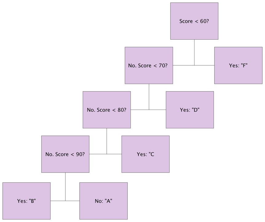
Suppose we want to create a variable called grades that is assigned as follows:
"F" if final_score <60
"D" if 60≤final_score<70
"C" if 70≤final_score<80
"B" if 80≤final_score<90
"A" if 90≤final_score
We can use a "nested" ifelse command as follows:
grade<-ifelse(final_score<60,"F", ifelse (final_score<70,"D", ifelse(final_score<80,"C", ifelse (final_score<90,"B", "A"))))
The logic by which this will assign grades is depicted in the figure below.
This type of scheme is really useful for putting different colors in graphs for different conditions. Consider the following graph of air quality measurements taken hourly in Beijing.
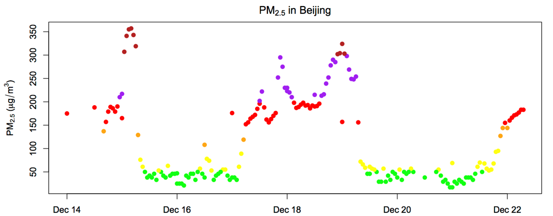
The code for the color section of the graph in the plot() command reads:
col = ifelse(pm25<=50,"green",
ifelse(pm25<101,"yellow",
ifelse(pm25<150,"orange",
ifelse(pm25<201,"red",
ifelse(pm25<301,"purple",
"firebrick")
)
)
)
)
There is a for loop construction in R which has form
> for (name in expr_1) expr_2
where name is the loop variable. expr_1 is a vector expression, (often a sequence like 1:20), and expr_2 is often a grouped expression with its sub-expressions written in terms of the dummy name. expr_2 is repeatedly evaluated as name ranges through the values in the vector result of expr_1.
Suppose, based on the ozone measurements in the airquality data set, we want to figure out which days were good air quality days (1) or bad air quality (0), based on a cutoff of ozone levels above 60ppb. Let us create a new vector called "goodair", which stores the information on good and bad air-quality days. We can do this using a for loop.
> numdays = nrow(airquality)
> numdays
[1] 153
> goodair = numeric(numdays)
# creates an object which will store the vector
> for(i in 1:numdays)
if (airquality$Ozone[i] > 60) goodair[i] = 0 else goodair[i] = 1
## (Notice that we have an if statement here within a for loop.)
Does the command above work? Why/why not?
Let's check the Ozone variable. What do you notice below?
> airquality$Ozone
[1] 41 36 12 18 NA 28 23 19 8 NA 7 16 11 14 18 14 34 6
[19] 30 11 1 11 4 32 NA NA NA 23 45 115 37 NA NA NA NA NA
[37] NA 29 NA 71 39 NA NA 23 NA NA 21 37 20 12 13 NA NA NA
[55] NA NA NA NA NA NA NA 135 49 32 NA 64 40 77 97 97 85 NA
[73] 10 27 NA 7 48 35 61 79 63 16 NA NA 80 108 20 52 82 50
[91] 64 59 39 9 16 78 35 66 122 89 110 NA NA 44 28 65 NA 22
[109] 59 23 31 44 21 9 NA 45 168 73 NA 76 118 84 85 96 78 73
[127] 91 47 32 20 23 21 24 44 21 28 9 13 46 18 13 24 16 13
[145] 23 36 7 14 30 NA 14 18 20
When there are missing values, many operations in R fail. One way to get around this is to create a new data frame that deletes all the rows corresponding to observations with missing rows. This can be done by means of the command "na.omit"
> airqualfull = na.omit(airquality)
> dim(airqualfull)
[1] 111 6
> dim(airquality)
[1] 153 6
# How many cases were deleted because of missing data?
Sometimes deleting all cases with missing values is useful, and sometimes it is a horrible idea…
We could get around this without deleting missing cases with an ifelse statement within the for loop.
Now let's try doing this again with the data with the complete cases.
> numdays = nrow(airqualfull)
> numdays
[1] 111
> goodair = numeric(numdays) # initialize the vector
> for(i in 1:numdays)
if (airqualfull$Ozone[i] >60) goodair[i] = 0 else goodair[i] = 1
> goodair
[1] 1 1 1 1 1 1 1 1 1 1 1 1 1 1 1 1 1 1 1 1 1 1 0 1 1 0 1 1 1 1 1 1 1 0 1 1 0
[38] 1 0 0 0 0 1 1 1 1 1 0 0 0 1 0 0 1 1 0 1 0 1 1 1 1 0 0 0 1 1 0 1 1 1 1 1 1
[75] 1 1 0 0 0 0 0 0 0 0 0 0 1 1 1 1 1 1 1 1 1 1 1 1 1 1 1 1 1 1 1 1 1 1 1 1 1
At this point we might be interested in which days were the ones with good air quality. The "which" command returns a set of indices corresponding to the condition specified. We can then use the indices to find the day of the month this corresponds to.
> which(goodair == 1) ## notice the double "=" signs!
> goodindices <- which(goodair == 1)
> airqualfull[goodindices,]
|
Suppose we want to define a day with good quality air as one with ozone levels below 60ppb, and temperatures less than 80 degrees F. Write an R loop to do this, and output the resulting subset of the data to a file called goodquality.txt. (Hint: use an ifelse() statement inside the for loop.) |
Similar to a loop function, the while statement can be used to perform an operation while a given condition is true. For example:
z <-0
while (z<5){
z<-z+2
print(z)
}
[1] 2
[1] 4
[1] 6
In the above while statement we initiate z to have a value of 0. We then state that as long as z is less than 5 we will continue to perform the following loop operation z<-z+2.
Thus we have
z <- 0+2 ##Initially z is 0, but after the first iteration of the loop the value of z is 2
z <- 2+2 ## After the second iteration the value of z is 4
z <- 4+2 ## After the third iteration the value of z is 6
The while statement stops here because now z is now bigger than 5.
Another option for looping is the repeat function. An example follows:
> i<-1
> repeat{
+ print(i)
+ if( i == 15) break
+ i<-i+1
+ }
[1] 1
[1] 2
[1] 3
[1] 4
[1] 5
[1] 6
[1] 7
[1] 8
[1] 9
[1] 10
[1] 11
[1] 12
[1] 13
[1] 14
[1] 15
All of these examples are analogous to MACROS in SAS. We want to do something many times, without doing it by hand each time; we are automating the process.
These methods can be greatly expanded to do dynamic, efficient, extremely complicated operations. The idea of this section is really just to get you familiar with how these programs do complicated operations.
Data frames and matrices allow for conditional indexing in R, which is often very useful. Instead of creating the goodair vector using a loop, we could directly extract the good air quality days using conditional indexing, using the single command below:
> airqualfull[airqualfull$Ozone < 60,]
It is worthwhile to keep in mind that many things in R can be done avoiding loops, and using conditional indexing can save a lot of time and effort! However, there are other times when using loops may be the only (or best) way to do things.
Conditional indexing is also useful for extracting groups of data from data frames, or splitting data into groups according to some criterion (or data which is already grouped according to some factor). For example, to get sets of ozone measurements for days with temperatures higher and lower than 80 degrees F, we can use:
> split(airqualfull$Ozone, airqualfull$Temp < 80)
$`FALSE`
[1] 45 29 71 39 23 135 49 32 64 40 77 97 97 85 27 7 48 35
[19] 61 79 63 80 108 20 52 82 50 64 59 39 9 16 122 89 110 44
[37] 28 65 168 73 76 118 84 85 96 78 73 91 47 32 20 44 16 36
$`TRUE`
[1] 41 36 12 18 23 19 8 16 11 14 18 14 34 6 30 11 1 11
[19] 4 32 23 115 37 21 37 20 12 13 10 16 22 59 23 31 44 21
[37] 9 45 23 21 24 21 28 9 13 46 18 13 24 13 23 7 14 30
[55] 14 18 20
|
Using conditional indexing, write an R command to replicate the results of the preceding exercise questtion. (Hint: use single &, not double &&.) |
Note: This topic has a lot to it, so I only cover the basics. There are plenty of online resources to do this on your own. There won't be any homework questions on this section.
Say you have two datasets and you want to merge them based on an ID number. A simple example of merging these by variable ID follows:
> dataset.1<-matrix(c(1,13,12,1, 2,12,10,2, 3,13,9,1, 4,9,8,2, 5,3,7,3, 6,5,6,1, 7,6,5,2, 8,5,5,3), ncol=4, byrow=T)
>
> dataset.1<-data.frame(dataset.1)
> names(dataset.1)<-c("ID","read 1","read 2","read 3")
> dataset.1
ID read 1 read 2 read 3
1 1 13 12 1
2 2 12 10 2
3 3 13 9 1
4 4 9 8 2
5 5 3 7 3
6 6 5 6 1
7 7 6 5 2
8 8 5 5 3
> dataset.2<-matrix(c(1,12, 2,13, 3,3, 4,15, 5,31, 6,15, 7,4, 8,6), ncol=2, byrow=T)
>
> dataset.2<-data.frame(dataset.2)
> names(dataset.2)<-c("ID","read 4")
> dataset.2
ID read 4
1 1 12
2 2 13
3 3 3
4 4 15
5 5 31
6 6 15
7 7 4
8 8 6
> dataset.merged <- merge(dataset.1,dataset.2,by="ID")
> dataset.merged
ID read 1 read 2 read 3 read 4
1 1 13 12 1 12
2 2 12 10 2 13
3 3 13 9 1 3
4 4 9 8 2 15
5 5 3 7 3 31
6 6 5 6 1 15
7 7 6 5 2 4
8 8 5 5 3 6
Now, a nice simple example of many-to-one merging:
> library(reshape)
> my.test.2<-matrix(c(1,13,12,1, 1,12,10,2, 2,13,9,1, 2,9,8,2, 2,3,7,3, 3,5,6,1, 3,6,5,2, 3,5,5,3), ncol=4, byrow=T)
#create sample data
# convert to a dataframe, a more robust format
> my.test.2<-as.data.frame(my.test.2)
# add column names
> names(my.test.2)<-c("ID","read A","read B","visit")
# print it to get a look. This is in "long" format
> my.test.2
ID read A read B visit
1 1 13 12 1
2 1 12 10 2
3 2 13 9 1
4 2 9 8 2
5 2 3 7 3
6 3 5 6 1
7 3 6 5 2
8 3 5 5 3
# above is a matrix of repeated measures on the same patient seen during multiple visits. The function below coerces the data frame into a 'wide' format, with one row per individual, renaming variables to account for missing values.
> wide_mytest <- reshape(my.test.2, direction="wide",idvar="ID",timevar="visit")
>
> wide_mytest
ID read A.1 read B.1 read A.2 read B.2 read A.3 read B.3
1 1 13 12 12 10 NA NA
3 2 13 9 9 8 3 7
6 3 5 6 6 5 5 5
Finally, you have a matrix you want to sort from smallest to largest of a particular column, but you want to keep each row intact. Do the following:
> setwd("/Users/Avery/Documents/classes/Graduate/720 Intro to R/spring 2015/classes/wk3/sorting matrices")
> read.table("ZZ")
p result x1 x2
1 0.8417549 1 2 0.4213440
2 0.9136235 1 3 -0.6412975
3 0.8361460 0 2 0.3798271
4 0.9850423 1 4 -0.5625415
5 0.3114491 1 0 1.4566465
#note each row here starts with an assigned number; this is NOT an actual column of (1,2,3,…), it's just a row designation.
#now sort it via column named "p"
> ZZ[order(ZZ[,1]),]
# or:
> attach(ZZ)
> ZZ[order(p),]
p result x1 x2
5 0.3114491 1 0 1.4566465
3 0.8361460 0 2 0.3798271
1 0.8417549 1 2 0.4213440
2 0.9136235 1 3 -0.6412975
4 0.9850423 1 4 -0.5625415
Now the matrix is sorted by column "p" while keeping the structure of the dataframe.
The R language allows the user to create objects of mode function. These are true R functions that are stored in a special internal form and may be used in further expressions and so on. In the process, the language gains enormously in power, convenience and elegance, and learning to write useful functions is one of the main ways to make your use of R comfortable and productive.
It should be emphasized that most of the functions supplied as part of the R system, such as mean(), var(), dim() and so on, are themselves written in R and thus do not differ materially from user written functions.
A function is defined by an assignment of the form
> name <- function(arg_1, arg_2, ...) expression
The expression is an R expression, (usually a grouped expression), that uses the arguments, arg_i, to calculate some value. The value of the expression is the value returned by the function.
A call to the function then usually takes the form name(expr_1, expr_2, ...) and may occur anywhere a function call is legitimate.
As a first example, consider a function to calculate a one-sample t-statistic to test the null hypothesis that in the height and weight data set, the mean population weight is "x" lb, where "x" can be specified by the user. This is an artificial example, of course, since there are other, simpler ways of achieving the same end (we'll do this next class).
> onesam <- function(y1, x) {
n1 <- length(y1) ##sample size
yb1 <- mean(y1) ##mean of y1
s1 <- var(y1) ##variance of y1
tstat <- (yb1 - x)/sqrt(s1/n1)
##computing t-statistic = (mean-x)/SE
tstat
}
With this function defined, you could perform one-sample t-tests using a call such as
> t.statistic <- onesam(htwtdata$weight, 130); t.statistic
To check whether this function works, compare it to running the actual t-test function inbuilt in R:
> t.test(htwtdata$weight-130)
A function can be called within a loop, or can be applied to elements of a vector or matrix at once, making R very powerful to use. We will continue looking at similar examples throughout the course.
Another example:
min.max.range <- function(x){
minimum<- min(x)
r <- max(x) - min(x)
maximum <- max(x)
print(minimum)
print(maximum)
print(r)
}
vec.1<- c(10, 20, 50)
min.max.range(vec.1)
[1] 10
[1] 50
[1] 40
|
Write a function called summarystat, which returns the mean, median,and standard deviation of a set of numbers. |
Summary
Reading
Assignment