Data Presentation
Authors:
Josée Dupuis, PhD, Professor of Biostatistics, Boston University School of Public Health
Wayne LaMorte, MD, PhD, MPH, Professor of Epidemiology, Boston University School of Public Health
|
"Modern data graphics can do much more than simply substitute for small statistical tables. At their best, graphics are instruments for reasoning about quantitative information. Often the most effective was to describe, explore, and summarize a set of numbers - even a very large set - is to look at pictures of those numbers. Furthermore, of all methods for analyzing and communicating statistical information, well-designed data graphics are usually the simplest and at the same time the most powerful." Edward R. Tufte in the introduction to "The Visual Display of Quantitative Information" |
While graphical summaries of data can certainly be powerful ways of communicating results clearly and unambiguously in a way that facilitates our ability to think about the information, poorly designed graphical displays can be ambiguous, confusing, and downright misleading. The keys to excellence in graphical design and communication are much like the keys to good writing. Adhere to fundamental principles of style and communicate as logically, accurately, and clearly as possible. Excellence in writing is generally achieved by avoiding unnecessary words and paragraphs; it is efficient. In a similar fashion, excellence in graphical presentation is generally achieved by efficient designs that avoid unnecessary ink.
Excellence in graphical presentation depends on:
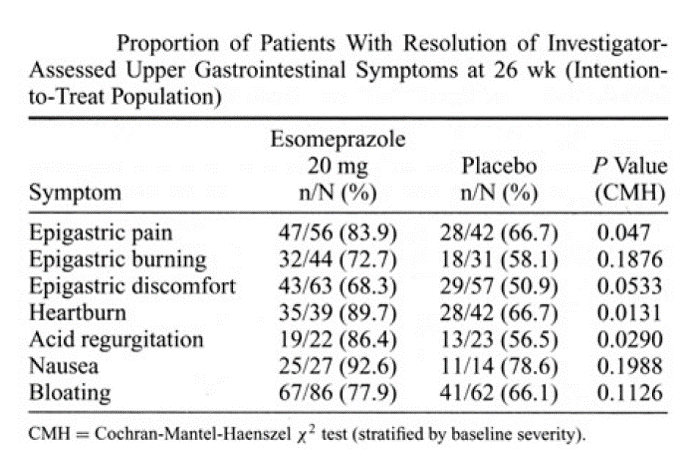
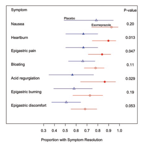
The side by side illustrations below show the same information, first in table form and then in graphical form. While the information in the table is precise, the real goal is to compare a series of clinical outcomes in subjects taking either a drug or a placebo. The graphical presentation on the right makes it possible to quickly see that for each of the outcomes evaluated, the drug produced relief in a great proportion of subjects. Moreover, the viewer gets a clear sense of the magnitude of improvement, and the error bars provided a sense of the uncertainty in the data.
|
Source: Connor JT. Statistical Graphics in AJG: Save the Ink for the Information. Am J of Gastroenterology. 2009; 104:1624-1630. |
|
Consider the data in the table below from http://www.cancer.gov/cancertopics/types/commoncancers
|
Type |
Incidence |
Proportion |
|---|---|---|
|
Bladder |
72,570 |
5.7% |
|
Breast |
232,340 |
18.2% |
|
Colon |
142,820 |
11.2% |
|
Kidney |
59,938 |
4.7% |
|
Leukemia |
48,610 |
3.8% |
|
Lung |
228,190 |
17.9% |
|
Melanoma |
76,690 |
6.0% |
|
Lymphoma |
69,740 |
5.5% |
|
Pancreas |
45,220 |
3.5% |
|
Prostate |
238,590 |
18.7% |
|
Thyroid |
60,220 |
4.7% |
Our ability to quickly understand the relative frequency of these cancers is hampered by presenting them in alphabetical order. It is much easier for the reader to grasp the relative frequency by listing them from most frequent to least frequent as in the next table.
|
Type |
Incidence |
Proportion |
|---|---|---|
|
Prostate |
238,590 |
18.7% |
|
Breast |
232,340 |
18.2% |
|
Lung |
228,340 |
17.9% |
|
Colon |
142,820 |
11.2% |
|
Melanoma |
76,690 |
6.0% |
|
Bladder |
72,570 |
5.7% |
|
Lymphoma |
69,740 |
5.5% |
|
Thyroid |
60,220 |
4.7% |
|
Kidney |
59,938 |
4.7% |
|
Leukemia |
48,610 |
3.8% |
|
Pancreas |
45,220 |
3.5% |
However, the same information might be presented more effectively with a dot plot, as shown below.
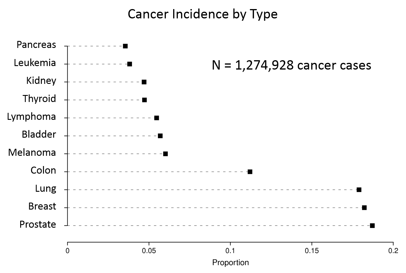
Data from http://www.cancer.gov/cancertopics/types/commoncancers
|
From E. R. Tufte. The Visual Display of Quantitative Information, 2nd Edition. Graphics Press, Cheshire, Connecticut, 2001.
|
Pattern perception is done by
Geographic Variation in Cancer
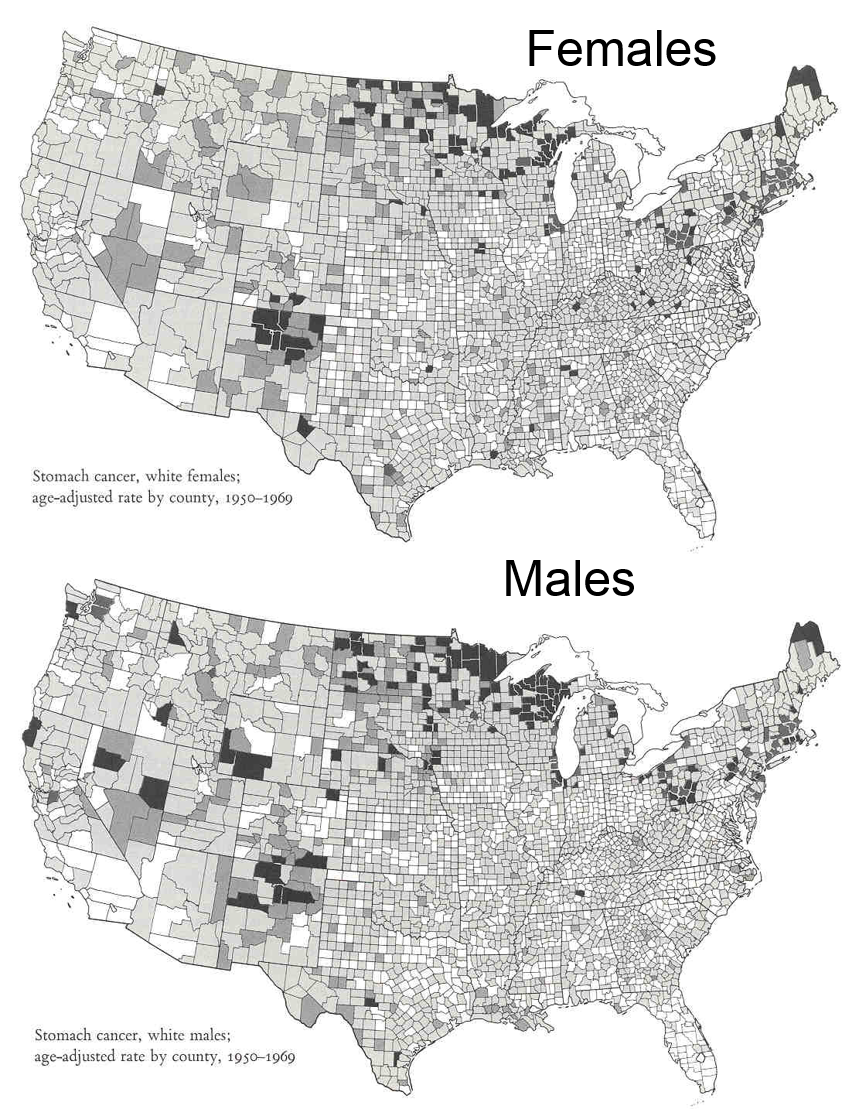
As an example, Tufte offers a series of maps that summarize the age-adjusted mortality rates for various types of cancer in the 3,056 counties in the United States. The maps showing the geographic variation in stomach cancer are shown below.
|
|
Adapted from Atlas of Cancer Mortality for U.S. Counties: 1950-1969, TJ Mason et al, PHS, NIH, 1975
|
These maps summarize an enormous amount of information and present it efficiently, coherently, and effectively.in a way that invites the viewer to make comparisons and to think about the substance of the findings. Consider, for example, that the region to the west of the Great Lakes was settled largely by immigrants from Germany and Scand anavia, where traditional methods of preserving food included pickling and curing of fish by smoking. Could these methods be associated with an increased risk of stomach cancer?
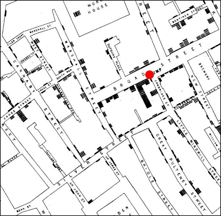
John Snow's Spot Map of Cholera Cases
Consider also the spot map that John Snow presented after the cholera outbreak in the Broad Street section of London in September 1854. Snow ascertained the place of residence or work of the victims and represented them on a map of the area using a small black disk to represent each victim and stacking them when more than one occurred at a particular location. Snow reasoned that cholera was probably caused by something that was ingested, because of the intense diarrhea and vomiting of the victims, and he noted that the vast majority of cholera deaths occurred in people who lived or worked in the immediate vicinity of the broad street pump (shown with a red dot that we added for clarity). He further ascertained that most of the victims drank water from the Broad Street pump, and it was this evidence that persuaded the authorities to remove the handle from the pump in order to prevent more deaths.
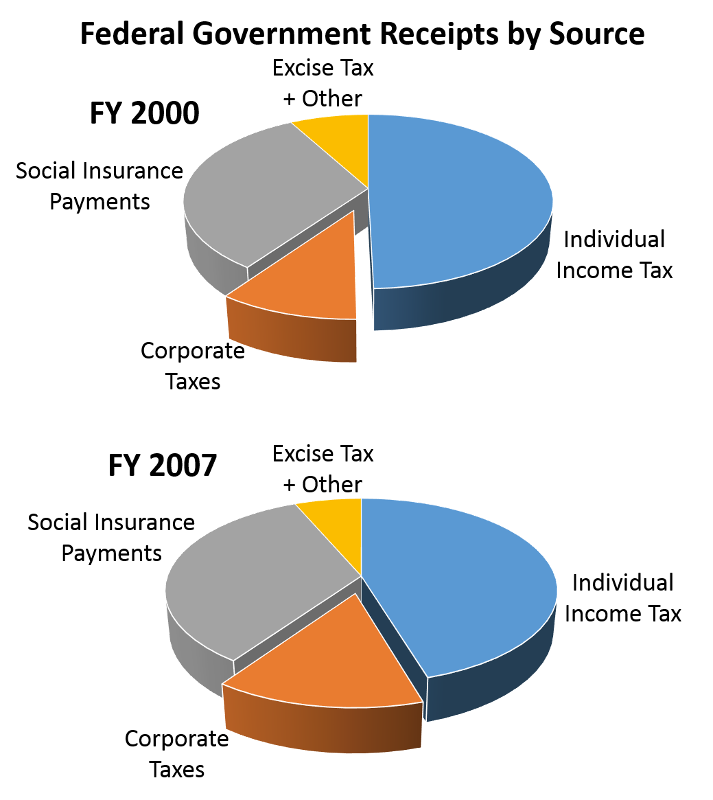
Humans can readily perceive differences like this when presented effectively as in the two previous examples. However, humans are not good at estimating differences without directly seeing them (especially for steep curves), and we are particularly bad at perceiving relative angles (the principal perception task used in a pie chart).
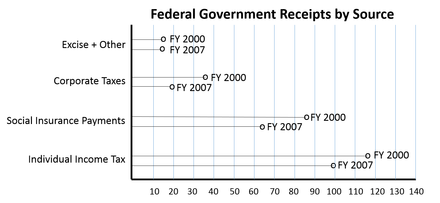
The use of pie charts is generally discouraged. Consider the pie chart on the left below. It is difficult to accurately assess the relative size of the components in the pie chart, because the human eye has difficulty judging angles. The dot plot on the right shows the same data, but it is much easier to quickly assess the relative size of the components and how they changed from Fiscal Year 2000 to Fiscal Year 2007.
|
|
Adapted from Wainer H.:Improving data displays: Ours and the media's. Chance, 2007;20:8-15. Data from http://www.taxpolicycenter.org/taxfacts/displayafact.cfm?Docid=203 |
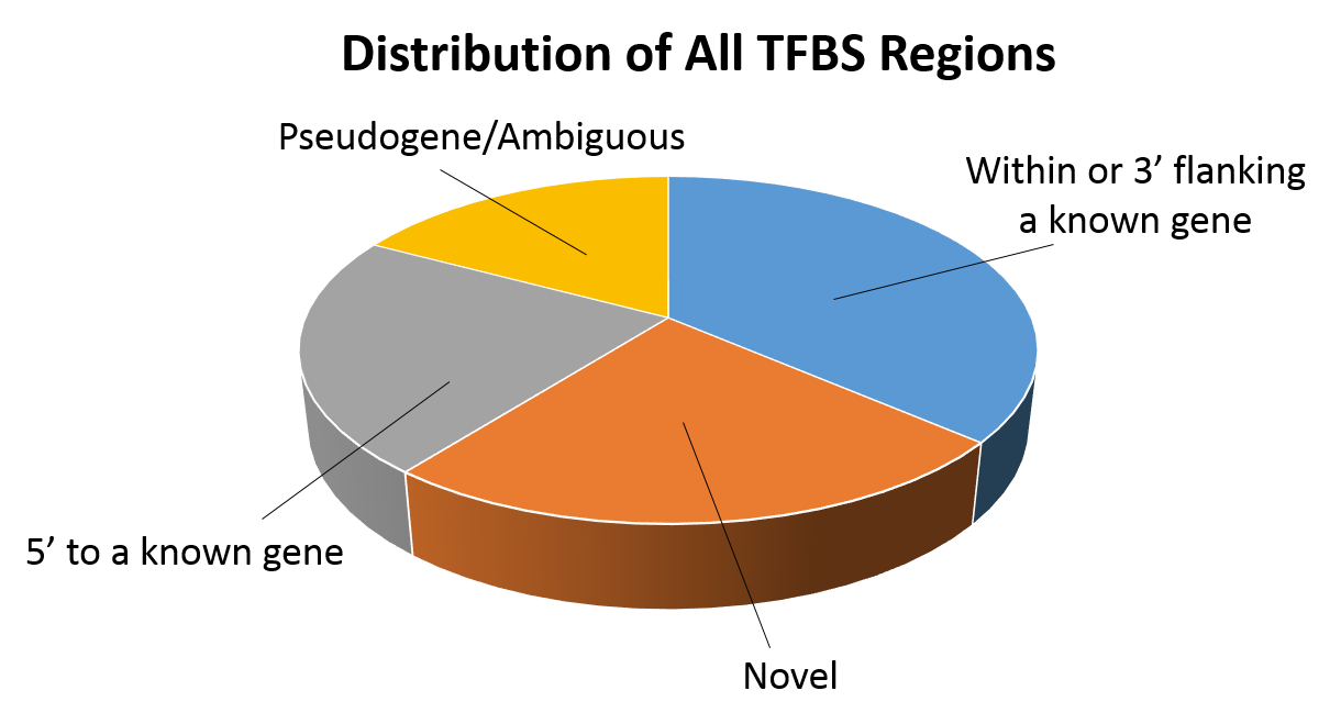
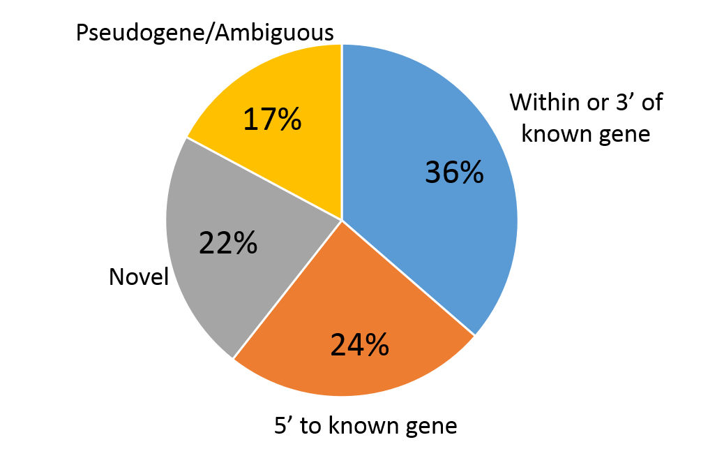
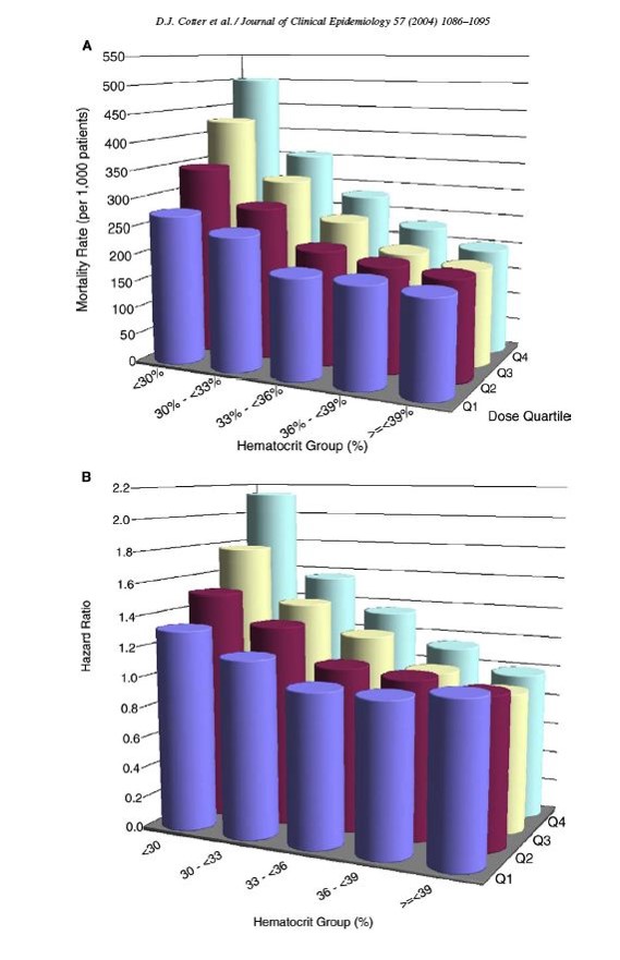
Consider the information in the two pie charts below (showing the same information).The 3-dimensional pie chart on the left distorts the relative proportions. In contrast the 2-dimensional pie chart on the right makes it much easier to compare the relative size of the varies components..
|
Adapted from Cawley S, et al. (2004) Unbiased mapping of transcription factor binding sites along human chromosomes 21 and 22 points to widespread regulation of noncoding RNAs. Cell 116:499-509, Figure 1 |
|
|
|
Adapted from Frank E. Harrell Jr. on graphics: http://biostat.mc.vanderbilt.edu/twiki/pub/Main/StatGraphCourse/graphscourse.pdf ] |
|
|
Source: Cotter DJ, et al. (2004) Hematocrit was not validated as a surrogate endpoint for survival among epoetin-treated hemodialysis patients. Journal of Clinical Epidemiology 57:1086-1095, Figure 2. |
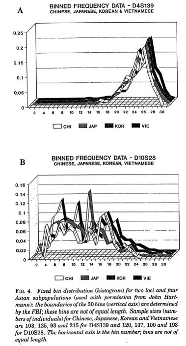
Source: Roeder K (1994) DNA fingerprinting: A review of the controversy (with discussion). Statistical Science 9:222-278, Figure 4. |
These 3-dimensional techniques distort the data and actually interfere with our ability to make accurate comparisons. The distortion caused by 3-dimensional elements can be particularly severe when the graphic is slanted at an angle or when the viewer tends to compare ends up unwittingly comparing the areas of the ink rather than the heights of the bars.
It is much easier to make comparisons with a chart like the one below.
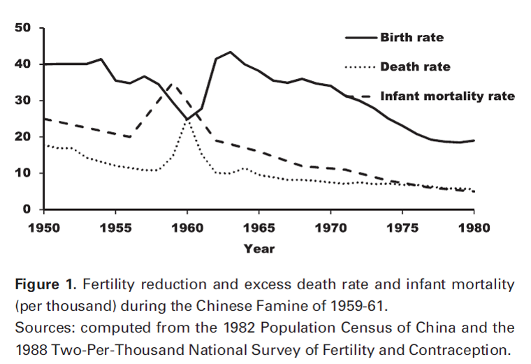
Source: Huang, C, Guo C, Nichols C, Chen S, Martorell R. Elevated levels of protein in urine in adulthood after exposure to
the Chinese famine of 1959–61 during gestation and the early postnatal period. Int. J. Epidemiol. (2014) 43 (6): 1806-1814 .
|
Consider these two examples.
|
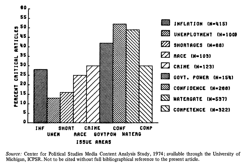
Hash lines are what E.R. Tufte refers to as "chart junk."
This graphic uses unnecessary bar graphs, pointless and annoying cross-hatching, and labels with incomplete abbreviations. The cluttered legend expands the inadequate bar labels, but it is difficult to go back and forth from the legend to the bar graph, and the use of all uppercase letters is visually unappealing. This presentation would have been greatly enhanced by simply using a horizontal dot plot that rank ordered the categories in a logical way. This approach could have been cleared and would have completely avoided the need for a legend. |
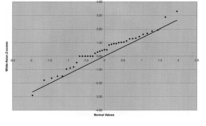
This grey background is a waste of ink, and it actually detracts from the readability of the graph by reducing contrast between the data points and other elements of the graph. Also, the axis labels are too small to be read easily. |
|
Source: Miller AH, Goldenberg EN, Erbring L. (1979) Type-Set Politics: Impact of Newspapers on Public Confidence. American Political Science Review, 73:67-84. |
Source: Jorgenson E, et al. (2005) Ethnicity and human genetic linkage maps. American Journal of Human Genetics 76:276-290, Figure 2 |
Here is a simple enumeration of the number of pets in a neighborhood. There is absolutely no reason to connect these counts with lines. This is, in fact, confusing and inappropriate and nothing more than "chart junk."
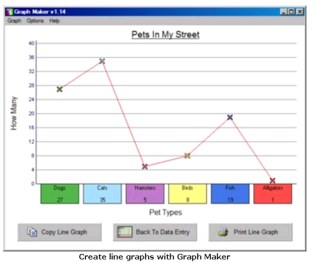
Source: http://www.go-education.com/free-graph-maker.html
Moiré effects are sometimes used in modern art to produce the appearance of vibration and movement. However, when these effects are applied to statistical presentations, they are distracting and add clutter because the visual noise interferes with the interpretation of the data.
Tufte presents the example shown below from Instituto de Expansao Commercial, Brasil, Graphicos Estatisticas (Rio de Janeiro, 1929, p. 15).
While the intention is to present quantitative information about the textile industry, the moiré effects do not add anything, and they are distracting, if not visually annoying.
|
Tips
|
Here is an attempt to compare catches of cod fish and crab across regions and to relate the variation to changes in water temperature. The problem here is that the Y-axes are vastly different, making it hard to sort out what's really going on. Even the Y-axes for temperature are vastly different.
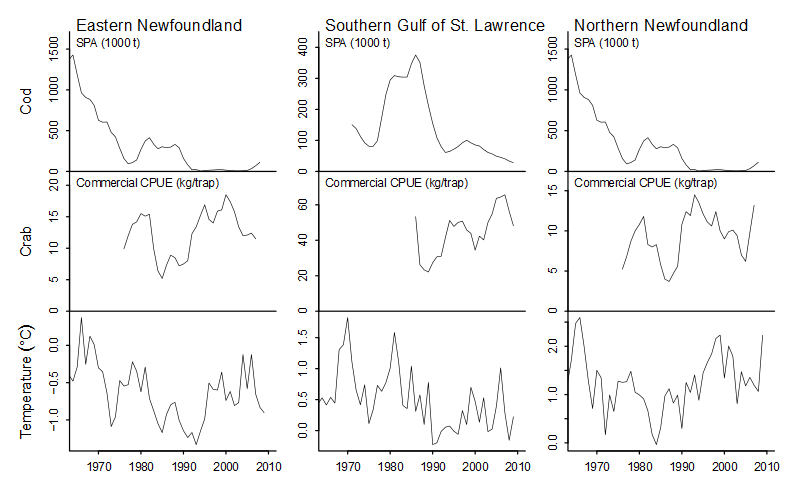
http://seananderson.ca/courses/11-multipanel/multipanel.pdf1
The ability to make comparisons is greatly facilitated by using the same scales for axes, as illustrated below.
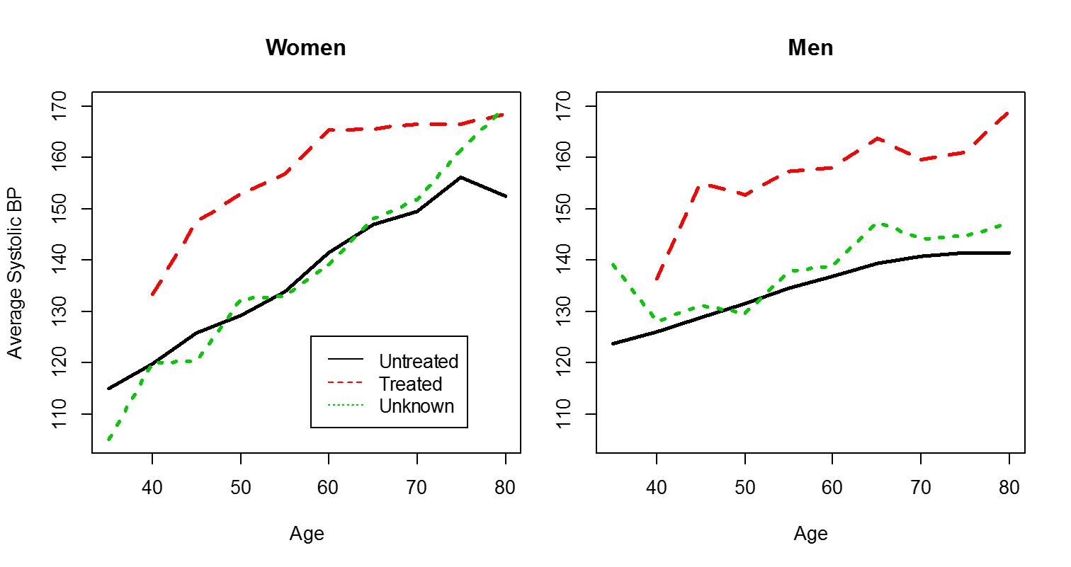
Data source: Dawber TR, Meadors GF, Moore FE Jr. Epidemiological approaches to heart disease:
the Framingham Study. Am J Public Health Nations Health. 1951;41(3):279-81. PMID: 14819398
It is also important to avoid distorting the X-axis. Note in the example below that the space between 0.05 to 0.1 is the same as space between 0.1 and 0.2.
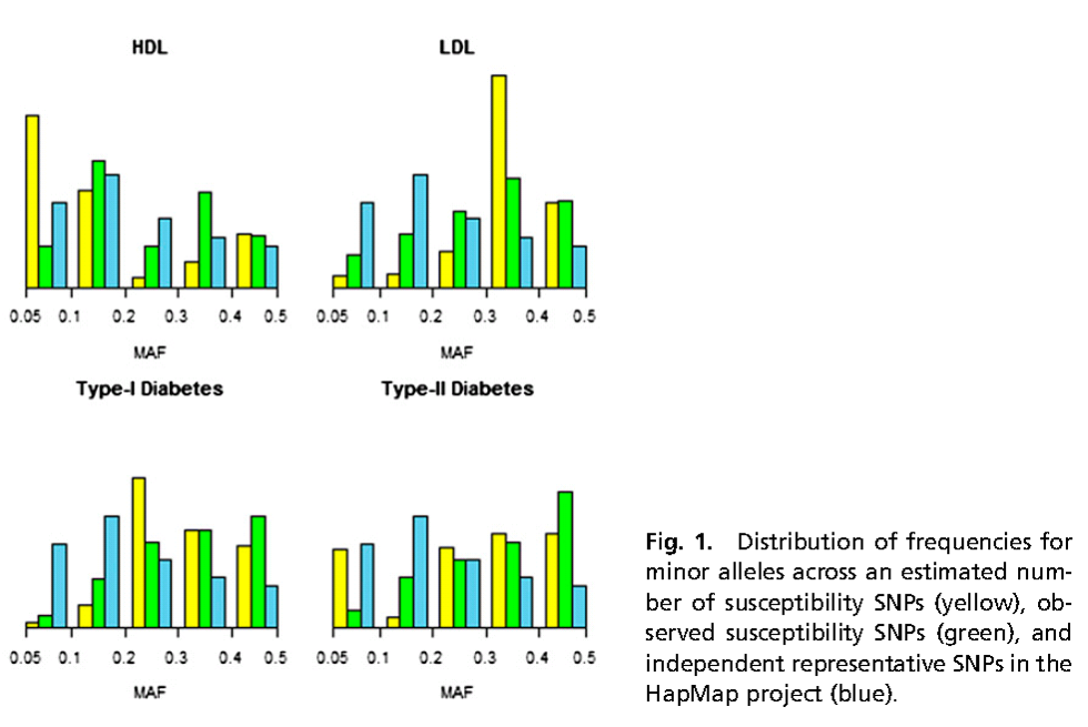
Source: Park JH, Gail MH, Weinberg CR, et al. Distribution of allele frequencies and effect sizes and
their interrelationships for common genetic susceptibility variants. Proc Natl Acad Sci U S A. 2011; 108:18026-31.
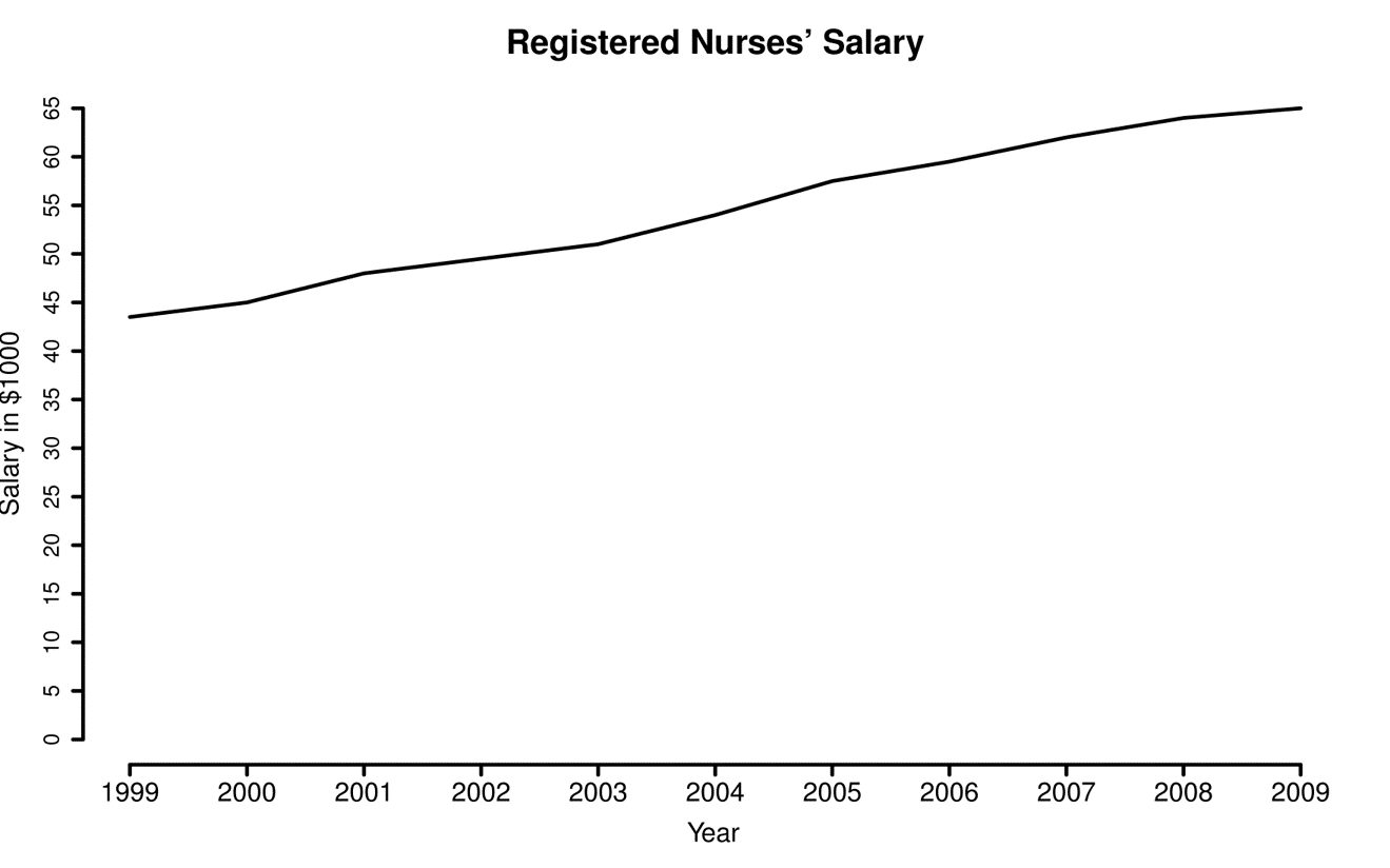
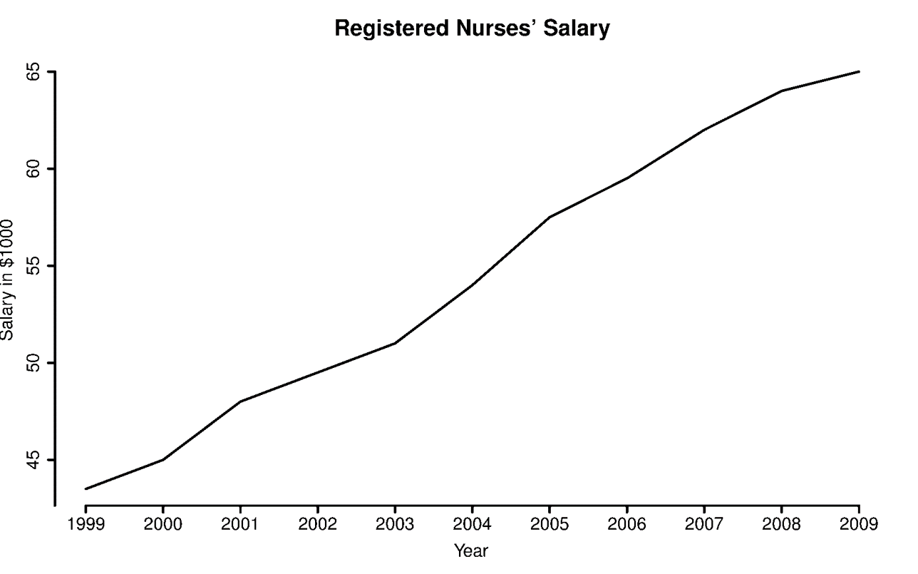
Consider the range of the Y-axis. In the examples below there is no relevant information below $40,000, so it is not necessary to begin the Y-axis at 0. The graph on the right makes more sense.
|
|
|
|
Data from http://www.myplan.com/careers/registered-nurses/salary-29-1111.00.html |
|
Also, consider using a log scale. this can be particularly useful when presenting ratios as in the example below.
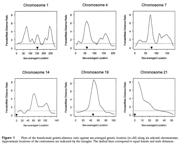
Source: Broman KW, Murray JC, Sheffield VC, White RL, Weber JL (1998) Comprehensive human genetic maps:
Individual and sex-specific variation in recombination. American Journal of Human Genetics 63:861-869, Figure 1
We noted earlier that pie charts make it difficult to see differences within a single pie chart, but this is particularly difficult when data is presented with multiple pie charts, as in the example below.
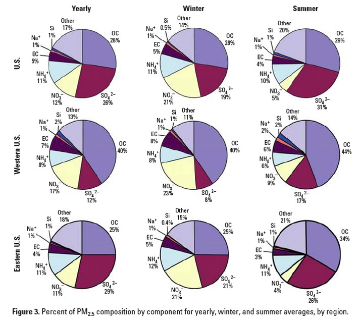
Source: Bell ML, et al. (2007) Spatial and temporal variation in PM2.5 chemical composition in the United States
for health effects studies. Environmental Health Perspectives 115:989-995, Figure 3
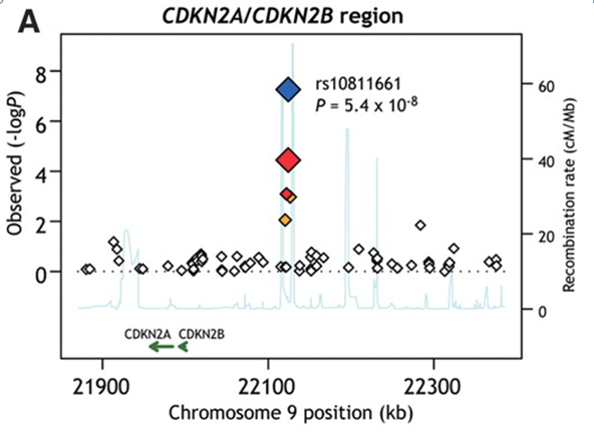
When multiple comparisons are being made, it is essential to use colors and symbols in a consistent way, as in this example.
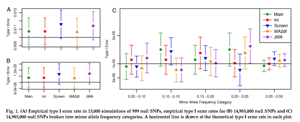
Source: Manning AK, LaValley M, Liu CT, et al. Meta-Analysis of Gene-Environment Interaction:
Joint Estimation of SNP and SNP x Environment Regression Coefficients. Genet Epidemiol 2011, 35(1):11-8.
Avoid putting too many lines on the same chart. In the example below, the only thing that is readily apparent is that 1980 was a very hot summer.
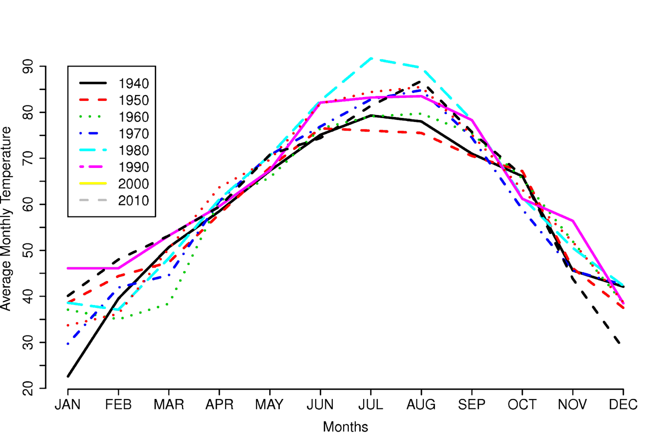
Data from National Weather Service Weather Forecast Office at
http://www.srh.noaa.gov/tsa/?n=climo_tulyeartemp
|
More Tips:
|
This isn't efficient, because this graphic is totally uninformative.
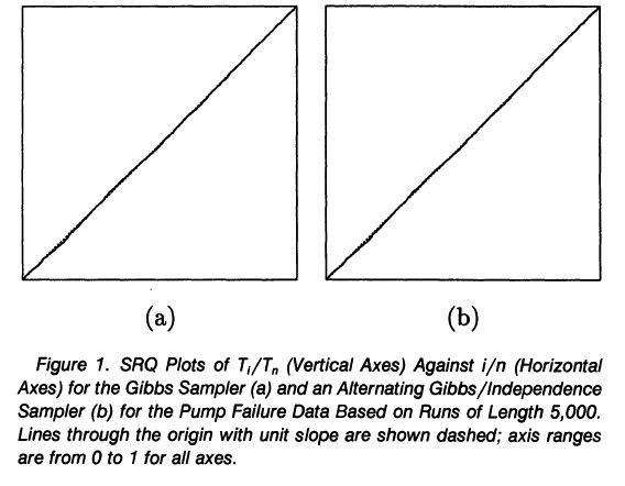
Source: Mykland P, Tierney L, Yu B (1995) Regeneration in Markov chain samplers. Journal of the American Statistical Association 90:233-241, Figure 1
|
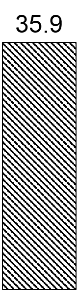
Bar charts are not appropriate for indicating means ± SEs. The only important information is the mean and the variation about the mean. Consider the figure to the right. By representing a mean with a number and a bar that has width, the information is representing one number over and over with:
|
|
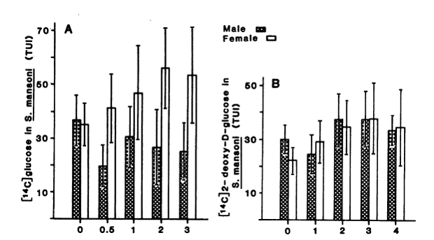
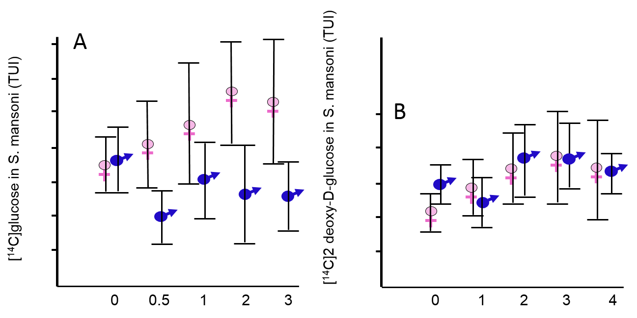
Bar graphs add ink without conveying any additional information, and they are distracting. The graph below on the left inappropriately uses bars which clutter the graph without adding anything. The graph on the right displays the same data, by does so more clearly and with less clutter.
|
Source: Conford EM, Huot ME. Glucose transfer from male to female schistosomes. Science. 1981 213:1269-71 |
|
|
"Just as a good editor of prose ruthlessly prunes unnecessary words, so a designer of statistical graphics should prune out ink that fails to present fresh data-information. Although nothing can replace a good graphical idea applied to an interesting set of numbers, editing and revision are as essential to sound graphical design work as they are to writing." Edward R. Tufte, "The Visual Display of Quantitative Information" |
|
|
|
>
|
Adapted from Frank E Harrell, Jr: on Graphics: http://biostat.mc.vanderbilt.edu/twiki/pub/Main/StatGraphCourse/graphscourse.pdf
|
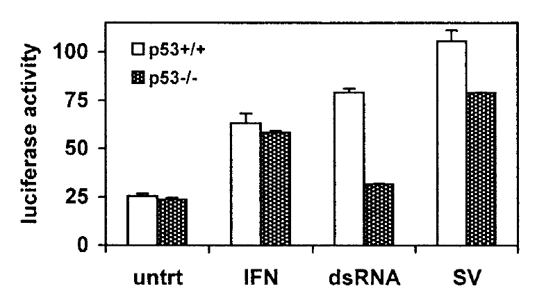
As noted previously, bar charts can be problematic. Here is another one presenting means and error bars, but the error bars are misleading because they only extend in one direction. A better alternative would have been to to use full error bars with a scatter plot, as illustrated previously (right).
|
Source: Hummer BT, Li XL, Hassel BA (2001) Role for p53 in gene induction by double-stranded RNA. J Virol 75:7774-7777, Figure 4 |
|
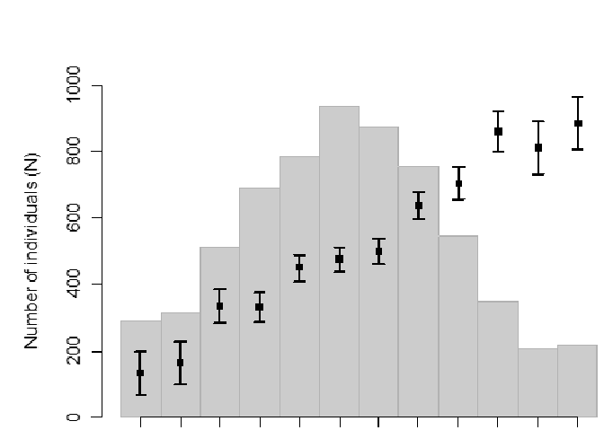
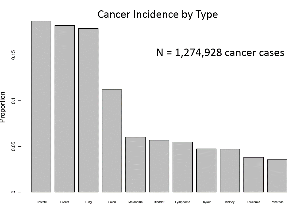
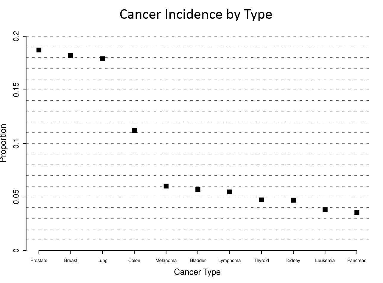
Consider the four graphs below presenting the incidence of cancer by type. The upper left graph unnecessary uses bars, which take up a lot of ink. This layout also ends up making the fonts for the types of cancer too small. Small font is also a problem for the dot plot at the upper right, and this one also has unnecessary grid lines across the entire width.
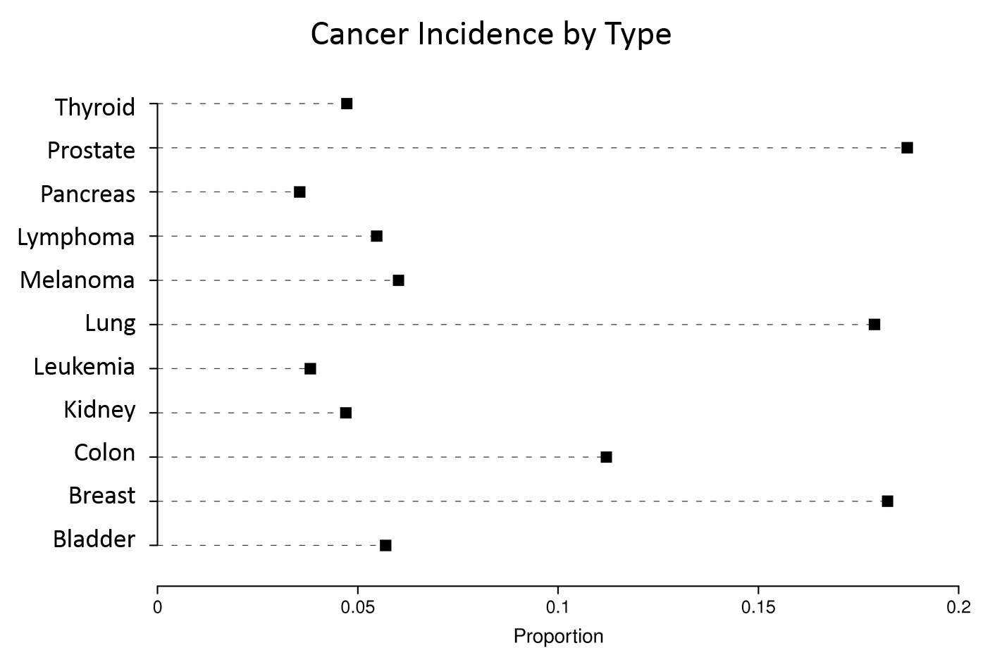
The graph at the lower left has more readable labels and uses a simple dot plot, but the rank order is difficult to figure out.
The graph at the lower right is clearly the best, since the labels are readable, the magnitude of incidence is shown clearly by the dot plots, and the cancers are sorted by frequency.
|
************************* + |
|
|
|
|
In this situation a cumulative distribution function conveys the most information and requires no grouping of the variable. A box plot will show selected quantiles effectively, and box plots are especially useful when stratifying by multiple categories of another variable.
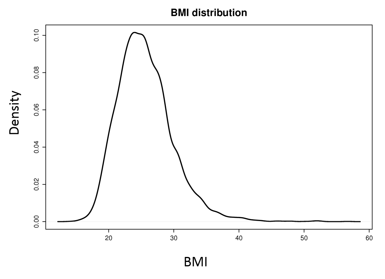
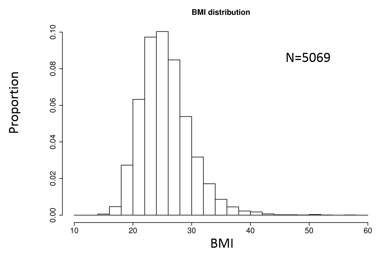
Histograms are also possible. Consider the examples below.
|
Density Plot |
Histogram |
Box Plot |
|
|
|
|
|
Adapted from Frank E. Harrell Jr. on graphics: http://biostat.mc.vanderbiltedu/twiki/pub/Main/StatGraphCourse/graphscourse.pdf Two categorical variables
Two continuous variables
|
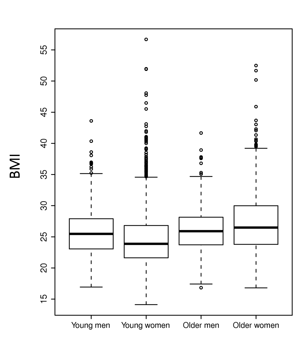
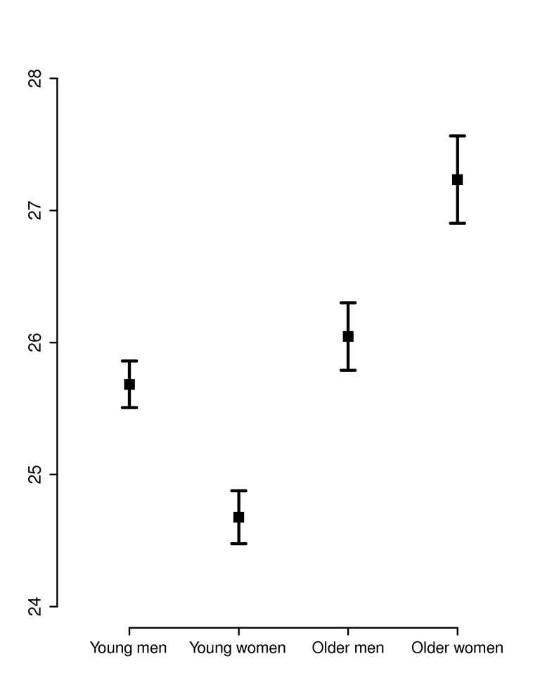
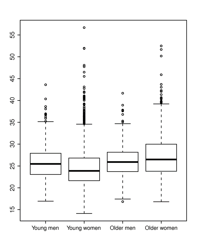
The two graphs below summarize BMI (Body Mass Index) measurements in four categories, i.e., younger and older men and women. The graph on the left shows the means and 95% confidence interval for the mean in each of the four groups. This is easy to interpret, but the viewer cannot see that the data is actually quite skewed. The graph on the right shows the same information presented as a box plot. With this presentation method one gets a better understanding of the skewed distribution and how the groups compare.
|
|
|
The next example is a scatter plot with a superimposed smoothed line of prediction. The shaded region embracing the blue line is a representation of the 95% confidence limits for the estimated prediction. This was created using "ggplot" in the R programming language.
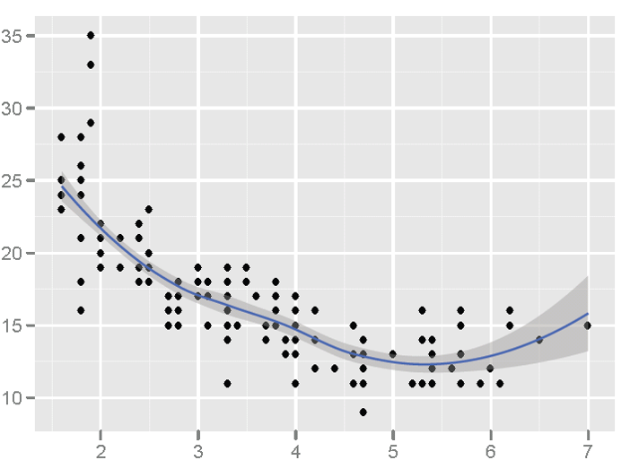
Source: Frank E. Harrell Jr. on graphics: http://biostat.mc.vanderbilt.edu/twiki/pub/Main/StatGraphCourse/graphscourse.pdf (page 121)
|
The example below shows the use of multiple panels.
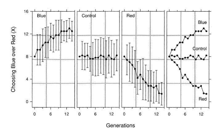
Source: Cleveland S. The Elements of Graphing Data. Hobart Press, Summit, NJ, 1994.
Options:
Confidence Limits
Source: Manning AK, LaValley M, Liu CT, et al. Meta-Analysis of Gene-Environment Interaction:
Joint Estimation of SNP and SNP x Environment Regression Coefficients. Genet Epidemiol 2011, 35(1):11-8.
Shaded Confidence Bands
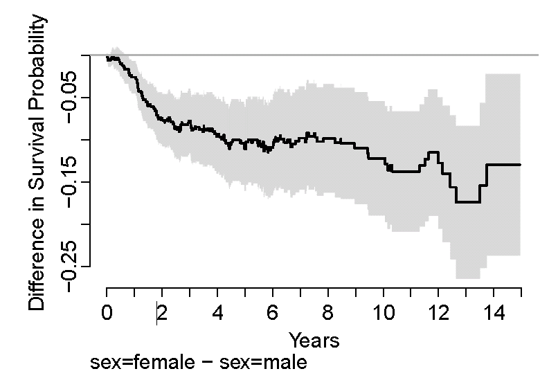
Source: Frank E. Harrell Jr. on graphics: http://biostat.mc.vanderbilt.edu/twiki/pub/Main/StatGraphCourse/graphscourse.pdf
Source: Tweedie RL and Mengersen KL. (1992) Br. J. Cancer 66: 700-705
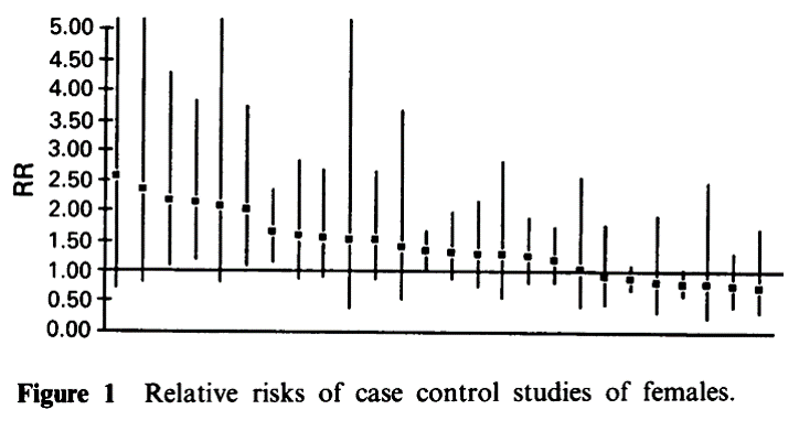
Forest Plot
This is a Forest plot summarizing 26 studies of cigarette smoke exposure on risk of lung cancer. The sizes of the black boxes indicating the estimated odds ratio are proportional to the sample size in each study.

Data from Tweedie RL and Mengersen KL. (1992) Br. J. Cancer 66: 700-705
Adapted from Wainer H. How to Display Data Badly. The American Statistician 1984; 38: 137-147.