Multivariable Methods
Previous modules discussed procedures for estimation and hypothesis testing and focused on whether a given outcome was associated with a single exposure or risk factor. However, many outcomes are influenced by more than a single exposure. There are several reasons for wanting to consider the effects of multiple variables on an outcome of interest.
For a more complete discussion of the phenomena of confounding and effect modification, please see the online module on these topics for the core course in epidemiology "Confounding and Effect Modification."
After completing this module, the student will be able to:
Confounding is a distortion (inaccuracy) in the estimated measure of association that occurs when the primary exposure of interest is mixed up with some other factor that is associated with the outcome.
There are three conditions that must be present for confounding to occur:
Since most health outcomes have multiple contributing causes, there are many possible confounders. For example, a study looking at the association between obesity and heart disease might be confounded by age, diet, smoking status, and a variety of other risk factors that might be unevenly distributed between the groups being compared.
Suppose a prospective cohort study was used to assess the association between obesity (defined as BMI > 30 at baseline) and the incidence of cardiovascular disease. Data are collected on participants between the ages of 35 and 65 who are initially free of cardiovascular disease (CVD) and followed over ten years. The table below summarizes the findings.
|
|
Incident CVD |
No CVD |
Total |
|
Obese |
46 |
254 |
300 |
|
Not Obese |
60 |
640 |
700 |
|
Total |
106 |
894 |
1,000 |
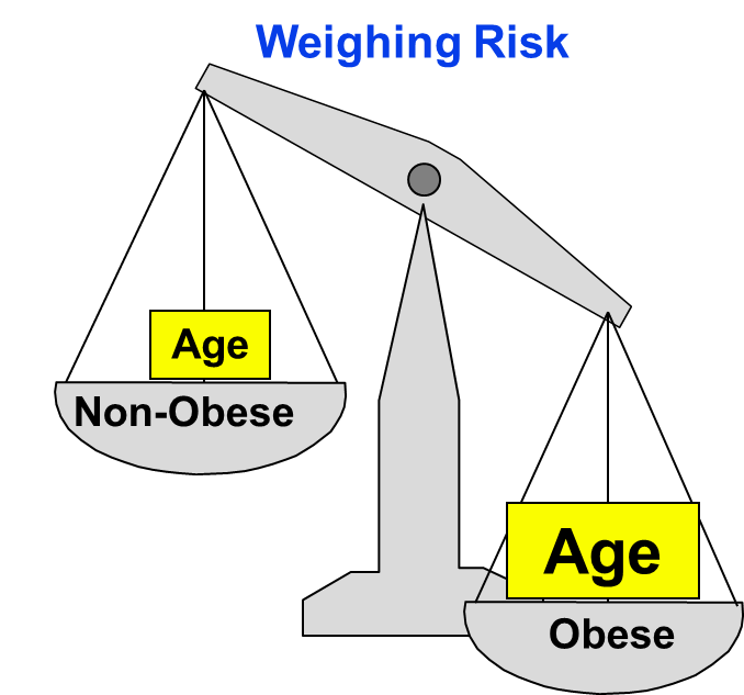
The cumulative incidence of CVD in obese persons) is 46/300 = 0.1533, and the cumulative incidence in non-obese persons is 60/700 = 0.0857. The estimated risk ratio for CVD in obese as compared to non-obese persons is RR = 0.153/0.86 = 1.79, suggesting that obese persons are 1.79 times as likely to develop CVD compared to non-obese persons. However, it is well known that the risk of CVD also increases with age, and BMI tends to increase with age. Could any (or all) of the apparent association between obesity and incident CVD be attributable to age?
If the obese group in our sample is older than the non-obese group, then all or part of the increased CVD risk in obese persons could possibly due to the increase in age rather than their obesity. If age is another risk factor for CVD, and if obese and non-obese persons differ in age, then our estimate of the association between obesity and CVD will be overestimated, because of the additional burden of being older.
In fact, in this data set, subjects who were 50+ were more likely to be obese (200/400 = 0.500) as compared to subjects younger than (100/600=0.167), as demonstrated by the table below.
|
|
Obese |
Not Obese |
Total |
|
Age 50+ |
200 |
200 |
400 |
|
Age <50 |
100 |
500 |
600 |
|
Total |
300 |
700 |
1000 |
In addition, older subjects were more likely to develop CVD (65/400 = 0.1625 versus 45/600 = 0.075).
|
|
Incident CVD |
No CVD |
Total |
|
Age 50+ |
65 |
335 |
400 |
|
Age < 50 |
45 |
555 |
600 |
|
Total |
110 |
890 |
1000 |
Thus, age meets the definition of a confounder (i.e., it is associated with the primary risk factor(obesity) and the outcome (CVD).
There are different methods to determine whether a variable is a confounder or not.
Lisa: Is hypothesis testing really a good way to approach this? If the sample size is small, hypothesis testing might fail to reject the null hypothesis, but there still might be confounding.
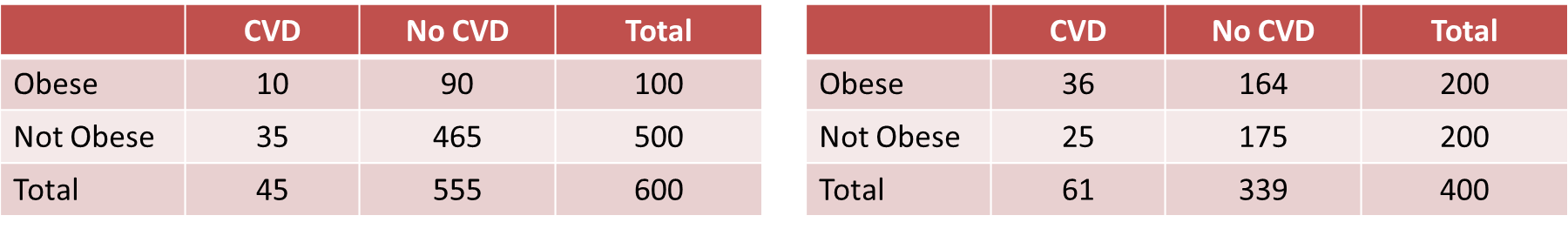
One way of identifying confounding is to examine the primary association of interest at different levels of a potential confounding factor. The side by side tables below examine the relationship between obesity and incident CVD in persons less than 50 years of age and in persons 50 years of age and older, separately.
|
Baseline Obesity and Incident CVD by Age Group |
|
|
Age < 50 |
Age 50+ |
|
|
|
|
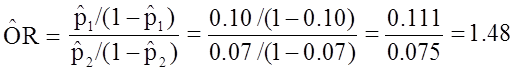
Among those < 50, the risk ratio is: RR = (10/100) / (35/500) = 0.100/0.070 = 1.43 |
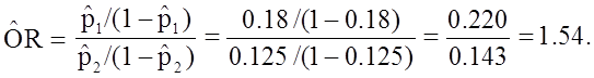
Among those 50+, the risk ratio is: RR = (36/200) / 25/200 = 0.180 / 0.125 = 1.44 |
Recall that the risk ratio for the total combined sample was RR = 1.79; this is sometimes referred to as the "crude" measure of association, because it is not adjusted for potential confounding factors. The risk ratios for the age-stratified analysis are similar to each other (RR = 1.43 and 1.44, respectively), but less than the crude risk ratio. This indicates that there was confounding by age in the overall sample. We saw that obese subjects more likely to be older than 50, and we also saw that those over age 50 had a greater risk of CVD. As a result, the crude analysis overestimated the true association between obesity (per se) and CVD, because of the greater proportion of older subjects among the obese group.
In the example above we saw that the relationship between obesity and CVD was confounded by age. When all of the data was pooled, it appeared that the risk ratio for the association between obesity and CVD was 1.79. However, when we stratified the analysis into those age <50 and those age 50+, we saw that both groups had a risk ratio of about 1.43. The distortion was due to the fact that obese individuals tended to be older, and older age is an independent risk factor for CVD. Consequently, in the analysis using the combined data set, the obese group had the added burden of an additional risk factor.
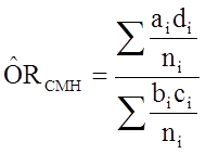
The Cochran-Mantel-Haenszel method is a technique that generates an estimate of an association between an exposure and an outcome after adjusting for or taking into account confounding. The method is used with a dichotomous outcome variable and a dichotomous risk factor. We stratify the data into two or more levels of the confounding factor (as we did in the example above). In essence, we create a series of two-by-two tables showing the association between the risk factor and outcome at two or more levels of the confounding factor, and we then compute a weighted average of the risk ratios or odds ratios across the strata (i.e., across subgroups or levels of the confounder).
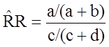
Before computing a Cochran-Mantel-Haenszel Estimate, it is important to have a standard layout for the two by two tables in each stratum. We will use the general format depicted here:
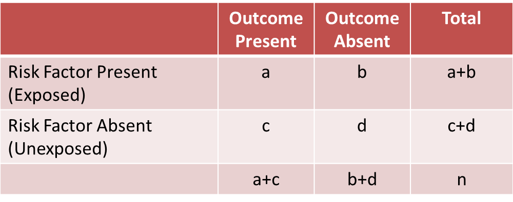
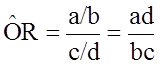
Using the notation in this table estimates for a risk ratio or an odds ratio would be computed as follows:
|
Risk Ratio
|
Odds Ratio
|
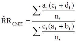
To explore and adjust for confounding, we can use a stratified analysis in which we set up a series of two-by-two tables, one for each stratum (category) of the confounding variable. Having done that, we can compute a weighted average of the estimates of the risk ratios or odds ratios across the strata. The weighted average provides a measure of association that is adjusted for confounding. The weighted averages for risk ratios and odds ratios are computed as follows:
|
Cochran-Mantel-Haenszel Estimate for a Risk Ratio |
Cochran-Mantel-Haenszel Estimate for an Odds Ratio |
|---|---|
|
|
|
Where ai, bi, ci and di are the numbers of participants in the cells of the two-by-two table in the ith stratum of the confounding variable. ni represents the number of participants in the ith stratum.
To illustrate the computations, we can use the previous example examining the association between obesity and CVD, which we stratified into two categories: those with age <50 and those who were 50+ at baseline:
|
Baseline Obesity and Incident CVD by Age Group |
|
|
Age < 50 |
Age 50+ |
|
|
|
|
Among those < 50, the risk ratio is: RR = (10/100) / (35/500) = 0.100/0.070 = 1.43 |
Among those 50+, the risk ratio is: RR = (36/200) / 25/200 = 0.180 / 0.125 = 1.44 |
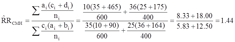
From the stratified data we can also compute the Cochran-Mantel-Haenszel estimate for the risk ratio as follows:
If we chose to, we could also use the same data set to compute a crude odds ratio (crude OR = 1.93) and we could also compute stratum-specific odds ratios as follows:
|
Among people of age <50 the odds ratio is:
|
Among people whose age was 50+ the odds ratio is:
|
And, using the same data we could also compute the Cochran-Mantel-Haenszel estimate for the odds ratio as follows:
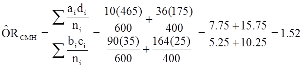
The Cochran-Mantel-Haenszel method produces a single, summary measure of association which accounts for the fact that there is a different association in each age stratum. Notice that the adjusted relative risk and adjusted odds ratio, 1.44 and 1.52, are not equal to the unadjusted or crude relative risk and odds ratio, 1.78 and 1.93. The adjustment for age produces estimates of the relative risk and odds ratio that are much closer to the stratum-specific estimates (the adjusted estimates are weighted averages of the stratum-specific estimates).
Effect modification occurs when the magnitude of the effect of the primary exposure on an outcome (i.e., the association) differs depending on the level of a third variable. In this situation, computing an overall estimate of association is misleading. One common way of dealing with effect modification is examine the association separately for each level of the third variable. For example, suppose a clinical trial is conducted and the drug is shown to result in a statistically significant reduction in total cholesterol. However, suppose that with closer scrutiny of the data, the investigators find that the drug is only effective in subjects with a specific genetic marker and that there is no effect in persons who do not possess the marker. The effect of the treatment is different depending on the presence or absence of the genetic marker. This is an example of effect modification or "interaction".
Unlike confounding, effect modification is a biological phenomenon in which the exposure has a different impact in different circumstances. Another good example is the effect of smoking on risk of lung cancer. Smoking and exposure to asbestos are both risk factors for lung cancer. Non-smokers exposed to asbestos have a 3-4 fold increased risk of lung cancer, and most studies suggest that smoking increases the risk of lung cancer about 20 times. However, shipyard workers who chronically inhaled asbestos fibers and also smoked had about a 64-fold increased risk of lung cancer. In other words, the effects of smoking and asbestos were not just additive – they were multiplicative. This suggests synergism or interaction, i.e., that the effect of smoking is somehow magnified in people who have also been exposed to asbestos. Multivariable methods can also be used to assess effect modification.
A stratified analysis provides a way to identify effect modification. Recall that on the previous page we used a stratified analysis to identify confounding. When there is just confounding, the measures of association in the subgroups will differ from the crude measure of association, but the measures of association across the subgroups will be similar. In contrast, when there is effect modification, the measures of association in the subgroups differ from one another.
For a more complete discussion of the phenomena of confounding and effect modification, please see the online module on these topics for the core course in epidemiology "Confounding and Effect Modification."
Evaluation of a Drug to Increase HDL Cholesterol
Consider the following clinical trial conducted to evaluate the efficacy of a new drug to increase HDL cholesterol (the "good" cholesterol). One hundred patients are enrolled in the trial and randomized to receive either the new drug or a placebo. Background characteristics (e.g., age, sex, educational level, income) and clinical characteristics (e.g., height, weight, blood pressure, total and HDL cholesterol levels) are measured at baseline, and they are found to be comparable in the two comparison groups. Subjects are instructed to take the assigned medication for 8 weeks, at which time their HDL cholesterol is measured again. The results are shown in the table below.
|
|
Sample Size |
Mean HDL |
Standard Deviation of HDL |
|
New Drug |
50 |
40.16 |
4.46 |
|
Placebo |
50 |
39.21 |
3.91 |
On average, the mean HDL levels are 0.95 units higher in patients treated with the new medication. A two sample test to compare mean HDL levels between treatments has a test statistic of Z = -1.13 which is not statistically significant at α=0.05.
Based on their preliminary studies, the investigators had expected a statistically significant increase in HDL cholesterol in the group treated with the new drug, and they wondered whether another variable might be masking the effect of the treatment. Other studies had, if fact, suggested that the effectiveness of a similar drug was différèrent in men and women. In this study, there are 19 men and 81 women. The table below shows the number and percent of men assigned to each treatment.
|
|
Sample Size |
Number (%) of Men |
|
New Drug |
50 |
10 (20%) |
|
Placebo |
50 |
9 (18%) |
There is no meaningful difference in the proportions of men assigned to receive the new drug or the placebo, so sex cannot be a a confounder here, since it does not differed in the treatment groups. However, when the data are stratified by sex, they find the following:
|
WOMEN |
Sample Size |
Mean HDL |
Standard Deviation of HDL |
|
New Drug |
40 |
38.88 |
3.97 |
|
Placebo |
41 |
39.24 |
4.21 |
|
|
|
|
|
|
MEN |
|
|
|
|
New Drug |
10 |
45.25 |
1.89 |
|
Placebo |
9 |
39.06 |
2.22 |
On average, the mean HDL levels are very similar in treated and untreated women, but the mean HDL levels are 6.19 units higher in men treated with the new drug. This is an example of effect modification by sex, i.e., the effect of the drug on HDL cholesterol is is different for men and women. In this case there is no apparent effect in women, but there appears to be a moderately large effect in men. (Note, however, that the comparison in men is based on a very small sample size, so this difference should be interpreted cautiously, since it could be the result of random error or confounding.
It is also important to note, that in the clinical trials setting, the only analyses that should be conducted are those that are planned a priori and specified in the study protocol. In contrast, in epidemiologic studies there are often exploratory analyses that are conducted to fully understand associations (or lack thereof). However, these analyses should also be restricted to those that are biologically sensible.
LISA: [ When you say "epidemiologic studies" here, do you really mean observational studies, i.e., case-control studies and cohort studies as opposed to randomized clinical trials? I'm also not sure why this statement is here at all. It some out of place, and perhaps should be included elsewhere.]
When there is effect modification, analysis of the pooled data can be misleading. In this example, the pooled data (men and women combined), shows no effect of treatment. Because there is effect modification by sex, it is important to look at the differences in HDL levels among men and women, considered separately. In stratified analyses, however, investigators must be careful to ensure that the sample size is adequate to provide a meaningful analysis.
In this section we will first discuss correlation analysis, which is used to quantify the association between two continuous variables (e.g., between an independent and a dependent variable or between two independent variables). Regression analysis is a related technique to assess the relationship between an outcome variable and one or more risk factors or confounding variables. The outcome variable is also called the response or dependent variable and the risk factors and confounders are called the predictors, or explanatory or independent variables. In regression analysis, the dependent variable is denoted "y" and the independent variables are denoted by "x".
[NOTE: The term "predictor" can be misleading if it is interpreted as the ability to predict even beyond the limits of the data. Also, the term "explanatory variable" might give an impression of a causal effect in a situation in which inferences should be limited to identifying associations. The terms "independent" and "dependent" variable are less subject to these interpretations as they do not strongly imply cause and effect.
In correlation analysis, we estimate a sample correlation coefficient, more specifically the Pearson Product Moment correlation coefficient. The sample correlation coefficient, denoted r,
ranges between -1 and +1 and quantifies the direction and strength of the linear association between the two variables. The correlation between two variables can be positive (i.e., higher levels of one variable are associated with higher levels of the other) or negative (i.e., higher levels of one variable are associated with lower levels of the other).
The sign of the correlation coefficient indicates the direction of the association. The magnitude of the correlation coefficient indicates the strength of the association.
For example, a correlation of r = 0.9 suggests a strong, positive association between two variables, whereas a correlation of r = -0.2 suggest a weak, negative association. A correlation close to zero suggests no linear association between two continuous variables.
LISA: [I find this description confusing. You say that the correlation coefficient is a measure of the "strength of association", but if you think about it, isn't the slope a better measure of association? We use risk ratios and odds ratios to quantify the strength of association, i.e., when an exposure is present it has how many times more likely the outcome is. The analogous quantity in correlation is the slope, i.e., for a given increment in the independent variable, how many times is the dependent variable going to increase? And "r" (or perhaps better R-squared) is a measure of how much of the variability in the dependent variable can be accounted for by differences in the independent variable. The analogous measure for a dichotomous variable and a dichotomous outcome would be the attributable proportion, i.e., the proportion of Y that can be attributed to the presence of the exposure.]
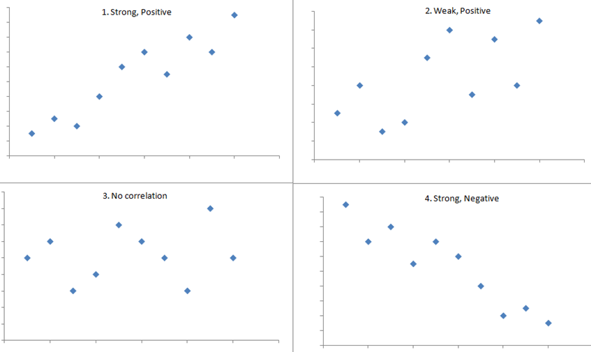
It is important to note that there may be a non-linear association between two continuous variables, but computation of a correlation coefficient does not detect this. Therefore, it is always important to evaluate the data carefully before computing a correlation coefficient. Graphical displays are particularly useful to explore associations between variables.
The figure below shows four hypothetical scenarios in which one continuous variable is plotted along the X-axis and the other along the Y-axis.
|
|
A small study is conducted involving 17 infants to investigate the association between gestational age at birth, measured in weeks, and birth weight, measured in grams.
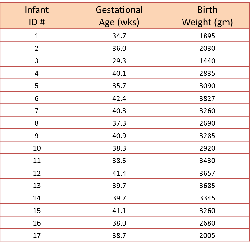
We wish to estimate the association between gestational age and infant birth weight. In this example, birth weight is the dependent variable and gestational age is the independent variable. Thus y=birth weight and x=gestational age. The data are displayed in a scatter diagram in the figure below.
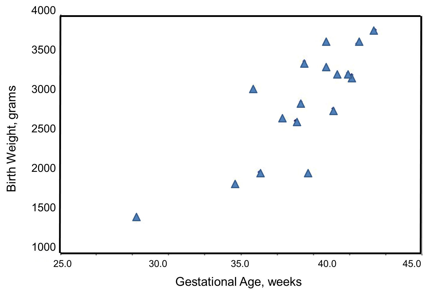
Each point represents an (x,y) pair (in this case the gestational age, measured in weeks, and the birth weight, measured in grams). Note that the independent variable is on the horizontal axis (or X-axis), and the dependent variable is on the vertical axis (or Y-axis). The scatter plot shows a positive or direct association between gestational age and birth weight. Infants with shorter gestational ages are more likely to be born with lower weights and infants with longer gestational ages are more likely to be born with higher weights.
The formula for the sample correlation coefficient is
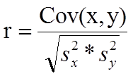
where Cov(x,y) is the covariance of x and y defined as
![]()
![]() are the sample variances of x and y, defined as
are the sample variances of x and y, defined as
![]()
The variances of x and y measure the variability of the x scores and y scores around their respective sample means (
![]() , considered separately). The covariance measures the variability of the (x,y) pairs around the mean of x and mean of y, considered simultaneously.
, considered separately). The covariance measures the variability of the (x,y) pairs around the mean of x and mean of y, considered simultaneously.
To compute the sample correlation coefficient, we need to compute the variance of gestational age, the variance of birth weight and also the covariance of gestational age and birth weight.
We first summarize the gestational age data. The mean gestational age is:
![]()
To compute the variance of gestational age, we need to sum the squared deviations (or differences) between each observed gestational age and the mean gestational age. The computations are summarized below.
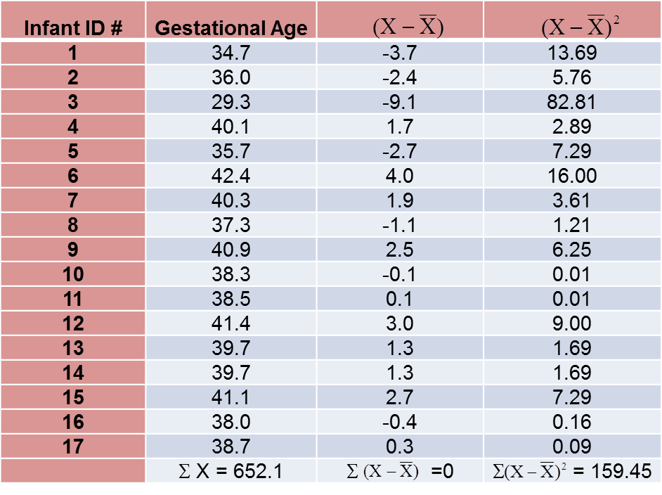
The variance of gestational age is:
![]()
Next, we summarize the birth weight data. The mean birth weight is:
![]()
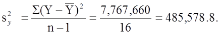
The variance of birth weight is computed just as we did for gestational age as shown in the table below.
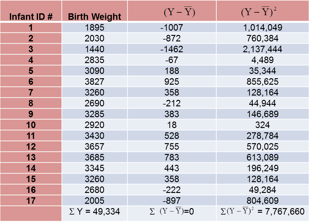
The variance of birth weight is:
Next we compute the covariance,
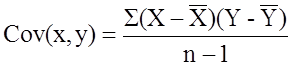
To compute the covariance of gestational age and birth weight, we need to multiply the deviation from the mean gestational age by the deviation from the mean birth weight for each participant (i.e.,
![]()
The computations are summarized below. Notice that we simply copy the deviations from the mean gestational age and birth weight from the two tables above into the table below and multiply.
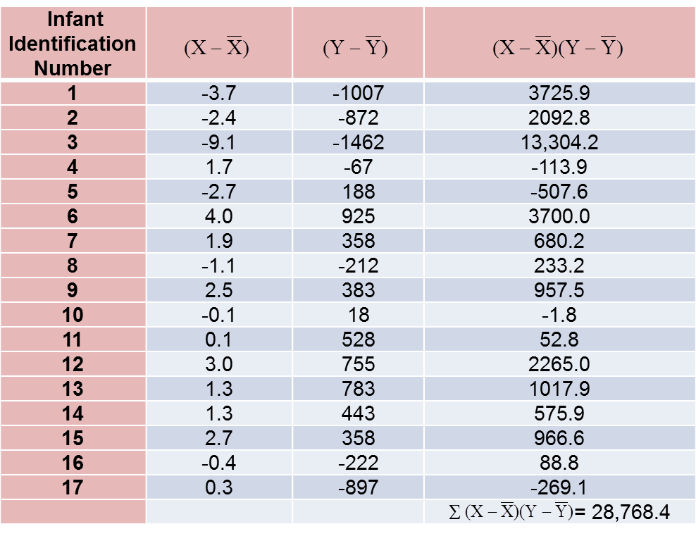
The covariance of gestational age and birth weight is:
![]()
We now compute the sample correlation coefficient:
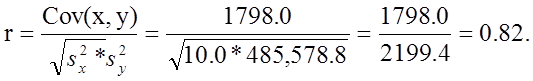
Not surprisingly, the sample correlation coefficient indicates a strong positive correlation.
As we noted, sample correlation coefficients range from -1 to +1. In practice, meaningful correlations (i.e., correlations that are clinically or practically important) can be as small as 0.4 (or -0.4) for positive (or negative) associations. There are also statistical tests to determine whether an observed correlation is statistically significant or not (i.e., statistically significantly different from zero). Procedures to test whether an observed sample correlation is suggestive of a statistically significant correlation are described in detail in Kleinbaum, Kupper and Muller.1
Regression analysis is a widely used technique which is useful for evaluating multiple independent variables. As a result, it is particularly useful for assess and adjusting for confounding. It can also be used to assess the presence of effect modification. Interested readers should see Kleinbaum, Kupper and Muller for more details on regression analysis and its many applications.1
Suppose we want to assess the association between total cholesterol and body mass index (BMI) in which total cholesterol is the dependent variable, and BMI is the independent variable. In regression analysis, the dependent variable is denoted Y and the independent variable is denoted X. So, in this case, Y=total cholesterol and X=BMI.
When there is a single continuous dependent variable and a single independent variable, the analysis is called a simple linear regression analysis. This analysis assumes that there is a linear association between the two variables. (If a different relationship is hypothesized, such as a curvilinear or exponential relationship, alternative regression analyses are performed.)
The figure below is a scatter diagram illustrating the relationship between BMI and total cholesterol. Each point represents the (X, Y) pair, in this case, BMI and the corresponding total cholesterol measured in each participant. Note that the independent variable is on the horizontal axis and the dependent variable on the vertical axis.
BMI and Total Cholesterol
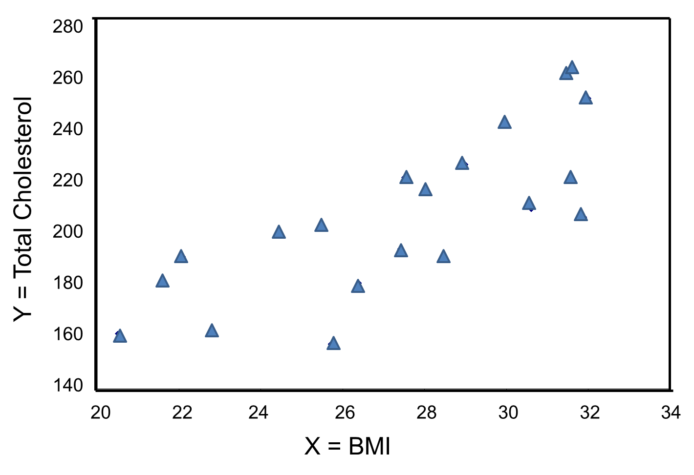
The graph shows that there is a positive or direct association between BMI and total cholesterol; participants with lower BMI are more likely to have lower total cholesterol levels and participants with higher BMI are more likely to have higher total cholesterol levels. In contrast, suppose we examine the association between BMI and HDL cholesterol.
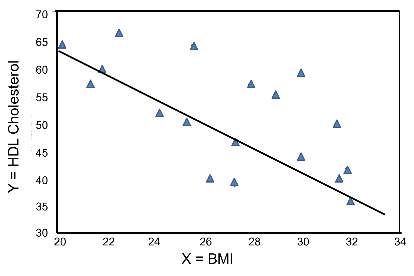
In contrast, the graph below depicts the relationship between BMI and HDL HDL cholesterol in the same sample of n=20 participants.
BMI and HDL Cholesterol
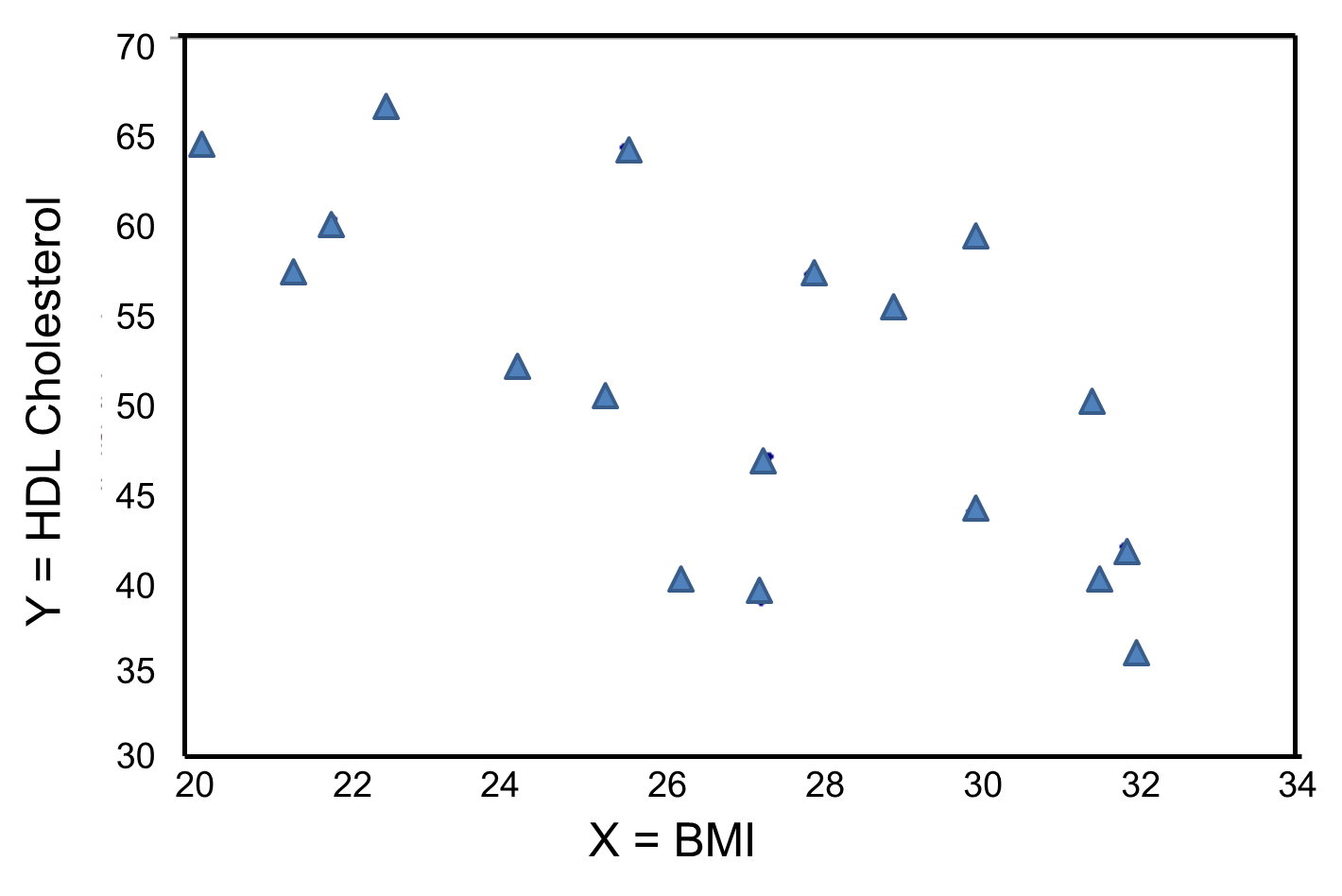
This graph shows a negative or inverse association between BMI and HDL cholesterol, i.e., those with lower BMI are more likely to have higher HDL cholesterol levels and those with higher BMI are more likely to have lower HDL cholesterol levels.
For either of these relationships we could use simple linear regression analysis to estimate the equation of the line that best describes the association between the independent variable and the dependent variable. The simple linear regression equation is as follows:
![]() , where
, where
![]() is the predicted or expected value of the outcome, X is the predictor , b0 is the estimated Y-intercept, and b1 is the estimated slope. The Y-intercept and slope are estimated from the sample data so as to minimize the sum of the squared differences between the observed and the predicted values of the outcome, i.e., the estimates minimize:
is the predicted or expected value of the outcome, X is the predictor , b0 is the estimated Y-intercept, and b1 is the estimated slope. The Y-intercept and slope are estimated from the sample data so as to minimize the sum of the squared differences between the observed and the predicted values of the outcome, i.e., the estimates minimize:
![]()
These differences between observed and predicted values of the outcome are called residuals. The estimates of the Y-intercept and slope minimize the sum of the squared residuals, and are called the least squares estimates.1
|
Residuals |
|---|
|
Conceptually, if the values of X provided a perfect prediction of Y then the sum of the squared differences between observed and predicted values of Y would be 0. That would mean that variability in Y could be completely explained by differences in X. However, if the differences between observed and predicted values are not 0, then we are unable to entirely account for differences in Y based on X, then there are residual errors in the prediction. The residual error could result from inaccurate measurements of X or Y, or there could be other variables besides X that affect the value of Y. |
Based on the observed data, the best estimate of a linear relationship will be obtained from an equation for the line that minimizes the differences between observed and predicted values of the outcome. The Y-intercept of this line is the value of the dependent variable (Y) when the independent variable (X) is zero. The slope of the line is the change in the dependent variable (Y) relative to a one unit change in the independent variable (X). The least squares estimates of the y-intercept and slope are computed as follows:
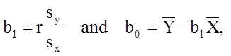
where
The least squares estimates of the regression coefficients, b 0 and b1, describing the relationship between BMI and total cholesterol are b0 = 28.07 and b1=6.49. These are computed as follows:

The estimate of the Y-intercept (b0 = 28.07) represents the estimated total cholesterol level when BMI is zero. Because a BMI of zero is meaningless, the Y-intercept is not informative. The estimate of the slope (b1 = 6.49) represents the change in total cholesterol relative to a one unit change in BMI. For example, if we compare two participants whose BMIs differ by 1 unit, we would expect their total cholesterols to differ by approximately 6.49 units (with the person with the higher BMI having the higher total cholesterol).
The equation of the regression line is as follows:
![]()
The graph below shows the estimated regression line superimposed on the scatter diagram.
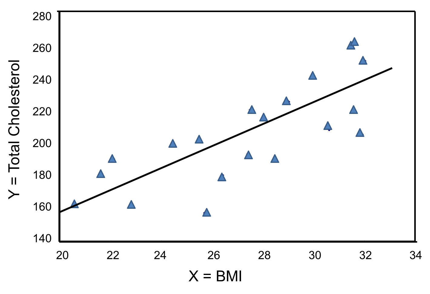
The regression equation can be used to estimate a participant's total cholesterol as a function of his/her BMI. For example, suppose a participant has a BMI of 25. We would estimate their total cholesterol to be 28.07 + 6.49(25) = 190.32. The equation can also be used to estimate total cholesterol for other values of BMI. However, the equation should only be used to estimate cholesterol levels for persons whose BMIs are in the range of the data used to generate the regression equation. In our sample, BMI ranges from 20 to 32, thus the equation should only be used to generate estimates of total cholesterol for persons with BMI in that range.
There are statistical tests that can be performed to assess whether the estimated regression coefficients (b0 and b1) are statistically significantly different from zero. The test of most interest is usually H0: b1=0 versus H1: b1≠0, where b1 is the population slope. If the population slope is significantly different from zero, we conclude that there is a statistically significant association between the independent and dependent variables.
The least squares estimates of the regression coefficients, b0 and b1, describing the relationship between BMI and HDL cholesterol are as follows: b0 = 111.77 and b1 = -2.35. These are computed as follows:

Again, the Y-intercept in uninformative because a BMI of zero is meaningless. The estimate of the slope (b1 = -2.35) represents the change in HDL cholesterol relative to a one unit change in BMI. If we compare two participants whose BMIs differ by 1 unit, we would expect their HDL cholesterols to differ by approximately 2.35 units (with the person with the higher BMI having the lower HDL cholesterol. The figure below shows the regression line superimposed on the scatter diagram for BMI and HDL cholesterol.
Linear regression analysis rests on the assumption that the dependent variable is continuous and that the distribution of the dependent variable (Y) at each value of the independent variable (X) is approximately normally distributed. Note, however, that the independent variable can be continuous (e.g., BMI) or can be dichotomous (see below).
We previously considered data from a clinical trial that evaluated the efficacy of a new drug to increase HDL cholesterol (see page 4 of this module). We compared the mean HDL levels between treatment groups using a two independent samples t test. Note, however, that regression analysis can also be used to compare mean HDL levels between treatments.
HDL cholesterol is the continuous dependent variable and treatment (new drug versus placebo) is the independent variable. A simple linear regression equation is estimated as follows:
![]() where
where
![]() is the estimated HDL level and X is a dichotomous variable (also called an indicator variable, i.e., indicating whether the active treatment was given or not). In this example, X is coded as 1 for participants who received the new drug and as 0 for participants who received the placebo.
is the estimated HDL level and X is a dichotomous variable (also called an indicator variable, i.e., indicating whether the active treatment was given or not). In this example, X is coded as 1 for participants who received the new drug and as 0 for participants who received the placebo.
The estimate of the Y-intercept is b0=39.21. The Y-intercept is the value of Y (HDL cholesterol) when X is zero. In this example, X=0 indicates the placebo group. Thus, the Y-intercept is exactly equal to the mean HDL level in the placebo group. The slope is b1=0.95. The slope represents the change in Y (HDL cholesterol) relative to a one unit change in X. A one unit change in X represents a difference in treatment assignment (placebo versus new drug). The slope represents the difference in mean HDL levels between the treatment groups. Dichotomous (or indicator) variables are usually coded as 0 or 1, where 0 is assigned to participants who do not have a particular risk factor, exposure or characteristic and 1 is assigned to participants who have the particular risk factor, exposure or characteristic. In a later section we will present multiple logistic regression analysis which applies in situations where the outcome is dichotomous (e.g., incident CVD).
There is convincing evidence that active smoking is a cause of lung cancer and heart disease. Many studies done in a wide variety of circumstances have consistently demonstrated a strong association and also indicate that the risk of lung cancer and cardiovascular disease (i.e.., heart attacks) increases in a dose-related way. These studies have led to the conclusion that active smoking is causally related to lung cancer and cardiovascular disease. Studies in active smokers have had the advantage that the lifetime exposure to tobacco smoke can be quantified with reasonable accuracy, since the unit dose is consistent (one cigarette) and the habitual nature of tobacco smoking makes it possible for most smokers to provide a reasonable estimate of their total lifetime exposure quantified in terms of cigarettes per day or packs per day. Frequently, average daily exposure (cigarettes or packs) is combined with duration of use in years in order to quantify exposure as "pack-years".
It has been much more difficult to establish whether environmental tobacco smoke (ETS) exposure is causally related to chronic diseases like heart disease and lung cancer, because the total lifetime exposure dosage is lower, and it is much more difficult to accurately estimate total lifetime exposure. In addition, quantifying these risks is also complicated because of confounding factors. For example, ETS exposure is usually classified based on parental or spousal smoking, but these studies are unable to quantify other environmental exposures to tobacco smoke, and inability to quantify and adjust for other environmental exposures such as air pollution makes it difficult to demonstrate an association even if one existed. As a result, there continues to be controversy over the risk imposed by environmental tobacco smoke (ETS). Some have gone so far as to claim that even very brief exposure to ETS can cause a myocardial infarction (heart attack), but a very large prospective cohort study by Estrom and Kabat was unable to demonstrate significant associations between exposure to spousal ETS and coronary heart disease, chronic obstructive pulmonary disease, or lung cancer. (It should be noted, however, that the report by Enstrom and Kabat has been widely criticized for methodologic problems, and these authors also had financial ties to the tobacco industry.)
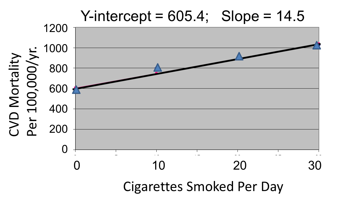
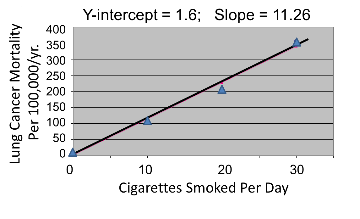
Correlation analysis provides a useful tool for thinking about this controversy. Consider data from the British Doctors Cohort. They reported the annual mortality for a variety of disease at four levels of cigarette smoking per day: Never smoked, 1-14/day, 15-24/day, and 25+/day. In order to perform a correlation analysis, I rounded the exposure levels to 0, 10, 20, and 30 respectively.
|
Cigarettes Smoked Per Day |
CVD Mortality/100,000 men/yr. |
Lung Cancer Mortality/100,000 men/yr. |
|---|---|---|
|
0 |
572 |
14 |
|
10 (actually 1-14) |
802 |
105 |
|
20 (actually 15-24) |
892 |
208 |
|
30 (actually >24) |
1025 |
355 |
The figures below show the two estimated regression lines superimposed on the scatter diagram. The correlation with amount of smoking was strong for both CVD mortality (r= 0.98) and for lung cancer (r = 0.99). Note also that the Y-intercept is a meaningful number here; it represents the predicted annual death rate from these disease in individuals who never smoked. The Y-intercept for prediction of CVD is slightly higher than the observed rate in never smokers, while the Y-intercept for lung cancer is lower than the observed rate in never smokers.
The linearity of these relationships suggests that there is an incremental risk with each additional cigarette smoked per day, and the additional risk is estimated by the slopes. This perhaps helps us think about the consequences of ETS exposure. For example, the risk of lung cancer in never smokers is quite low, but there is a finite risk; various reports suggest a risk of 10-15 lung cancers/100,000 per year. If an individual who never smoked actively was exposed to the equivalent of one cigarette's smoke in the form of ETS, then the regression suggests that their risk would increase by 11.26 lung cancer deaths per 100,000 per year. However, the risk is clearly dose-related. Therefore, if a non-smoker was employed by a tavern with heavy levels of ETS, the risk might be substantially greater.
|
|
|
Finally, it should be noted that some findings suggest that the association between smoking and heart disease is non-linear at the very lowest exposure levels, meaning that non-smokers have a disproportionate increase in risk when exposed to ETS due to an increase in platelet aggregation.
Multiple linear regression analysis is an extension of simple linear regression analysis, used to assess the association between two or more independent variables and a single continuous dependent variable. The multiple linear regression equation is as follows:
![]() ,
,
where![]() is the predicted or expected value of the dependent variable, X1 through Xp are p distinct independent or predictor variables, b0 is the value of Y when all of the independent variables (X1 through Xp) are equal to zero, and b1 through bp are the estimated regression coefficients. Each regression coefficient represents the change in Y relative to a one unit change in the respective independent variable. In the multiple regression situation, b1, for example, is the change in Y relative to a one unit change in X1, holding all other independent variables constant (i.e., when the remaining independent variables are held at the same value or are fixed). Again, statistical tests can be performed to assess whether each regression coefficient is significantly different from zero.
is the predicted or expected value of the dependent variable, X1 through Xp are p distinct independent or predictor variables, b0 is the value of Y when all of the independent variables (X1 through Xp) are equal to zero, and b1 through bp are the estimated regression coefficients. Each regression coefficient represents the change in Y relative to a one unit change in the respective independent variable. In the multiple regression situation, b1, for example, is the change in Y relative to a one unit change in X1, holding all other independent variables constant (i.e., when the remaining independent variables are held at the same value or are fixed). Again, statistical tests can be performed to assess whether each regression coefficient is significantly different from zero.
Multiple regression analysis is also used to assess whether confounding exists. Since multiple linear regression analysis allows us to estimate the association between a given independent variable and the outcome holding all other variables constant, it provides a way of adjusting for (or accounting for) potentially confounding variables that have been included in the model.
Suppose we have a risk factor or an exposure variable, which we denote X1 (e.g., X1=obesity or X1=treatment), and an outcome or dependent variable which we denote Y. We can estimate a simple linear regression equation relating the risk factor (the independent variable) to the dependent variable as follows:
![]()
where b1 is the estimated regression coefficient that quantifies the association between the risk factor and the outcome.
Suppose we now want to assess whether a third variable (e.g., age) is a confounder. We denote the potential confounder X2, and then estimate a multiple linear regression equation as follows:
![]() .
.
In the multiple linear regression equation, b1 is the estimated regression coefficient that quantifies the association between the risk factor X1 and the outcome, adjusted for X2 (b2 is the estimated regression coefficient that quantifies the association between the potential confounder and the outcome). As noted earlier, some investigators assess confounding by assessing how much the regression coefficient associated with the risk factor (i.e., the measure of association) changes after adjusting for the potential confounder. In this case, we compare b1 from the simple linear regression model to b1 from the multiple linear regression model. As a rule of thumb, if the regression coefficient from the simple linear regression model changes by more than 10%, then X2 is said to be a confounder.
Once a variable is identified as a confounder, we can then use multiple linear regression analysis to estimate the association between the risk factor and the outcome adjusting for that confounder. The test of significance of the regression coefficient associated with the risk factor can be used to assess whether the association between the risk factor is statistically significant after accounting for one or more confounding variables. This is also illustrated below.
Example - The Association Between BMI and Systolic Blood Pressure
Suppose we want to assess the association between BMI and systolic blood pressure using data collected in the seventh examination of the Framingham Offspring Study. A total of n=3,539 participants attended the exam, and their mean systolic blood pressure was 127.3 with a standard deviation of 19.0. The mean BMI in the sample was 28.2 with a standard deviation of 5.3.
A simple linear regression analysis reveals the following:
|
Independent Variable |
Regression Coefficient |
T |
P-value |
|
Intercept |
108.28 |
62.61 |
0.0001 |
|
BMI |
0.67 |
11.06 |
0.0001 |
The simple linear regression model is:
![]()
where
![]() is the predicted of expected systolic blood pressure. The regression coefficient associated with BMI is 0.67 suggesting that each one unit increase in BMI is associated with a 0.67 unit increase in systolic blood pressure. The association between BMI and systolic blood pressure is also statistically significant (p=0.0001).
is the predicted of expected systolic blood pressure. The regression coefficient associated with BMI is 0.67 suggesting that each one unit increase in BMI is associated with a 0.67 unit increase in systolic blood pressure. The association between BMI and systolic blood pressure is also statistically significant (p=0.0001).
Suppose we now want to assess whether age (a continuous variable, measured in years), male gender (yes/no), and treatment for hypertension (yes/no) are potential confounders, and if so, appropriately account for these using multiple linear regression analysis. For analytic purposes, treatment for hypertension is coded as 1=yes and 0=no. Gender is coded as 1=male and 0=female. A multiple regression analysis reveals the following:
| Independent Variable |
Regression Coefficient |
T |
P-value |
| Intercept |
68.15 |
26.33 |
0.0001 |
| BMI |
0.58 |
10.30 |
0.0001 |
| Age |
0.65 |
20.22 |
0.0001 |
| Male gender |
0.94 |
1.58 |
0.1133 |
| Treatment for hypertension |
6.44 |
9.74 |
0.0001 |
The multiple regression model is:
![]() = 68.15 + 0.58 (BMI) + 0.65 (Age) + 0.94 (Male gender) + 6.44 (Treatment for hypertension).
= 68.15 + 0.58 (BMI) + 0.65 (Age) + 0.94 (Male gender) + 6.44 (Treatment for hypertension).
Notice that the association between BMI and systolic blood pressure is smaller (0.58 versus 0.67) after adjustment for age, gender and treatment for hypertension. BMI remains statistically significantly associated with systolic blood pressure (p=0.0001), but the magnitude of the association is lower after adjustment. The regression coefficient decreases by 13%.
[Actually, doesn't it decrease by 15.5%. In this case the true "beginning value" was 0.58, and confounding caused it to appear to be 0.67. so the actual % change = 0.09/0.58 = 15.5%.]
Using the informal rule (i.e., a change in the coefficient in either direction by 10% or more), we meet the criteria for confounding. Thus, part of the association between BMI and systolic blood pressure is explained by age, gender and treatment for hypertension.
This also suggests a useful way of identifying confounding. Typically, we try to establish the association between a primary risk factor and a given outcome after adjusting for one or more other risk factors. One useful strategy is to use multiple regression models to examine the association between the primary risk factor and the outcome before and after including possible confounding factors. If the inclusion of a possible confounding variable in the model causes the association between the primary risk factor and the outcome to change by 10% or more, then the additional variable is a confounder.
Assessing only the p-values suggests that these three independent variables are equally statistically significant. The magnitude of the t statistics provides a means to judge relative importance of the independent variables. In this example, age is the most significant independent variable, followed by BMI, treatment for hypertension and then male gender. In fact, male gender does not reach statistical significance (p=0.1133) in the multiple regression model.
Some investigators argue that regardless of whether an important variable such as gender reaches statistical significance it should be retained in the model. Other investigators only retain variables that are statistically significant.
[Not sure what you mean here; do you mean to control for confounding?] /WL
This is yet another example of the complexity involved in multivariable modeling. The multiple regression model produces an estimate of the association between BMI and systolic blood pressure that accounts for differences in systolic blood pressure due to age, gender and treatment for hypertension.
A one unit increase in BMI is associated with a 0.58 unit increase in systolic blood pressure holding age, gender and treatment for hypertension constant. Each additional year of age is associated with a 0.65 unit increase in systolic blood pressure, holding BMI, gender and treatment for hypertension constant.
Men have higher systolic blood pressures, by approximately 0.94 units, holding BMI, age and treatment for hypertension constant and persons on treatment for hypertension have higher systolic blood pressures, by approximately 6.44 units, holding BMI, age and gender constant. The multiple regression equation can be used to estimate systolic blood pressures as a function of a participant's BMI, age, gender and treatment for hypertension status. For example, we can estimate the blood pressure of a 50 year old male, with a BMI of 25 who is not on treatment for hypertension as follows:
![]()
We can estimate the blood pressure of a 50 year old female, with a BMI of 25 who is on treatment for hypertension as follows:
![]()
On page 4 of this module we considered data from a clinical trial designed to evaluate the efficacy of a new drug to increase HDL cholesterol. One hundred patients enrolled in the study and were randomized to receive either the new drug or a placebo. The investigators were at first disappointed to find very little difference in the mean HDL cholesterol levels of treated and untreated subjects.
|
|
Sample Size |
Mean HDL |
Standard Deviation of HDL |
|
New Drug |
50 |
40.16 |
4.46 |
|
Placebo |
50 |
39.21 |
3.91 |
However, when they analyzed the data separately in men and women, they found evidence of an effect in men, but not in women. We noted that when the magnitude of association differs at different levels of another variable (in this case gender), it suggests that effect modification is present.
|
WOMEN |
Sample Size |
Mean HDL |
Standard Deviation of HDL |
|
New Drug |
40 |
38.88 |
3.97 |
|
Placebo |
41 |
39.24 |
4.21 |
|
|
|
|
|
|
MEN |
|
|
|
|
New Drug |
10 |
45.25 |
1.89 |
|
Placebo |
9 |
39.06 |
2.22 |
Multiple regression analysis can be used to assess effect modification. This is done by estimating a multiple regression equation relating the outcome of interest (Y) to independent variables representing the treatment assignment, sex and the product of the two (called the treatment by sex interaction variable). For the analysis, we let T = the treatment assignment (1=new drug and 0=placebo), M = male gender (1=yes, 0=no) and TM, i.e., T * M or T x M, the product of treatment and male gender. In this case, the multiple regression analysis revealed the following:
|
Independent Variable |
Regression Coefficient |
T |
P-value |
|
Intercept |
39.24 |
65.89 |
0.0001 |
|
T (Treatment) |
-0.36 |
-0.43 |
0.6711 |
|
M (Male Gender) |
-0.18 |
-0.13 |
0.8991 |
|
TM (Treatment x Male Gender) |
6.55 |
3.37 |
0.0011 |
The multiple regression model is:
![]()
The details of the test are not shown here, but note in the table above that in this model, the regression coefficient associated with the interaction term, b3, is statistically significant (i.e., H0: b3 = 0 versus H1: b3 ≠ 0). The fact that this is statistically significant indicates that the association between treatment and outcome differs by sex.
The model shown above can be used to estimate the mean HDL levels for men and women who are assigned to the new medication and to the placebo. In order to use the model to generate these estimates, we must recall the coding scheme (i.e., T = 1 indicates new drug, T=0 indicates placebo, M=1 indicates male sex and M=0 indicates female sex).
The expected or predicted HDL for men (M=1) assigned to the new drug (T=1) can be estimated as follows:
![]()
The expected HDL for men (M=1) assigned to the placebo (T=0) is:
![]()
Similarly, the expected HDL for women (M=0) assigned to the new drug (T=1) is:
![]()
The expected HDL for women (M=0)assigned to the placebo (T=0) is:
![]()
Notice that the expected HDL levels for men and women on the new drug and on placebo are identical to the means shown the table summarizing the stratified analysis. Because there is effect modification, separate simple linear regression models are estimated to assess the treatment effect in men and women:
|
MEN |
Regression Coefficient |
T |
P-value |
|
Intercept |
39.08 |
57.09 |
0.0001 |
|
T (Treatment) |
6.19 |
6.56 |
0.0001 |
|
|
|
|
|
|
WOMEN |
Regression Coefficient |
T |
P-value |
|
Intercept |
39.24 |
61.36 |
0.0001 |
|
T (Treatment) |
-0.36 |
-0.40 |
0.6927 |
The regression models are:
|
In Men:
|
In Women:
|
In men, the regression coefficient associated with treatment (b1=6.19) is statistically significant (details not shown), but in women, the regression coefficient associated with treatment (b1= -0.36) is not statistically significant (details not shown).
Multiple linear regression analysis is a widely applied technique. In this section we showed here how it can be used to assess and account for confounding and to assess effect modification. The techniques we described can be extended to adjust for several confounders simultaneously and to investigate more complex effect modification (e.g., three-way statistical interactions).
There is an important distinction between confounding and effect modification. Confounding is a distortion of an estimated association caused by an unequal distribution of another risk factor. When there is confounding, we would like to account for it (or adjust for it) in order to estimate the association without distortion. In contrast, effect modification is a biological phenomenon in which the magnitude of association is differs at different levels of another factor, e.g., a drug that has an effect on men, but not in women. In the example, present above it would be in inappropriate to pool the results in men and women. Instead, the goal should be to describe effect modification and report the different effects separately.
There are many other applications of multiple regression analysis. A popular application is to assess the relationships between several predictor variables simultaneously, and a single, continuous outcome. For example, it may be of interest to determine which predictors, in a relatively large set of candidate predictors, are most important or most strongly associated with an outcome. It is always important in statistical analysis, particularly in the multivariable arena, that statistical modeling is guided by biologically plausible associations.
Independent variables in regression models can be continuous or dichotomous. Regression models can also accommodate categorical independent variables. For example, it might be of interest to assess whether there is a difference in total cholesterol by race/ethnicity. The module on Hypothesis Testing presented analysis of variance as one way of testing for differences in means of a continuous outcome among several comparison groups. Regression analysis can also be used. However, the investigator must create indicator variables to represent the different comparison groups (e.g., different racial/ethnic groups). The set of indicator variables (also called dummy variables) are considered in the multiple regression model simultaneously as a set independent variables. For example, suppose that participants indicate which of the following best represents their race/ethnicity: White, Black or African American, American Indian or Alaskan Native, Asian, Native Hawaiian or Pacific Islander or Other Race. This categorical variable has six response options. To consider race/ethnicity as a predictor in a regression model, we create five indicator variables (one less than the total number of response options) to represent the six different groups. To create the set of indicators, or set of dummy variables, we first decide on a reference group or category. In this example, the reference group is the racial group that we will compare the other groups against. Indicator variable are created for the remaining groups and coded 1 for participants who are in that group (e.g., are of the specific race/ethnicity of interest) and all others are coded 0. In the multiple regression model, the regression coefficients associated with each of the dummy variables (representing in this example each race/ethnicity group) are interpreted as the expected difference in the mean of the outcome variable for that race/ethnicity as compared to the reference group, holding all other predictors constant. The example below uses an investigation of risk factors for low birth weight to illustrates this technique as well as the interpretation of the regression coefficients in the model.
An observational study is conducted to investigate risk factors associated with infant birth weight. The study involves 832 pregnant women. Each woman provides demographic and clinical data and is followed through the outcome of pregnancy. At the time of delivery, the infant s birth weight is measured, in grams, as is their gestational age, in weeks. Birth weights vary widely and range from 404 to 5400 grams. The mean birth weight is 3367.83 grams with a standard deviation of 537.21 grams. Investigators wish to determine whether there are differences in birth weight by infant gender, gestational age, mother's age and mother's race. In the study sample, 421/832 (50.6%) of the infants are male and the mean gestational age at birth is 39.49 weeks with a standard deviation of 1.81 weeks (range 22-43 weeks). The mean mother's age is 30.83 years with a standard deviation of 5.76 years (range 17-45 years). Approximately 49% of the mothers are white; 41% are Hispanic; 5% are black; and 5% identify themselves as other race. A multiple regression analysis is performed relating infant gender (coded 1=male, 0=female), gestational age in weeks, mother's age in years and 3 dummy or indicator variables reflecting mother's race. The results are summarized in the table below.
|
Independent Variable |
Regression Coefficient |
T |
P-value |
|
Intercept |
-3850.92 |
-11.56 |
0.0001 |
|
Male infant |
174.79 |
6.06 |
0.0001 |
|
Gestational age, weeks |
179.89 |
22.35 |
0.0001 |
|
Mother's age, years |
1.38 |
0.47 |
0.6361 |
|
Black race |
-138.46 |
-1.93 |
0.0535 |
|
Hispanic race |
-13.07 |
-0.37 |
0.7103 |
|
Other race |
-68.67 |
-1.05 |
0.2918 |
Many of the predictor variables are statistically significantly associated with birth weight. Male infants are approximately 175 grams heavier than female infants, adjusting for gestational age, mother's age and mother's race/ethnicity. Gestational age is highly significant (p=0.0001), with each additional gestational week associated with an increase of 179.89 grams in birth weight, holding infant gender, mother's age and mother's race/ethnicity constant. Mother's age does not reach statistical significance (p=0.6361). Mother's race is modeled as a set of three dummy or indicator variables. In this analysis, white race is the reference group. Infants born to black mothers have lower birth weight by approximately 140 grams (as compared to infants born to white mothers), adjusting for gestational age, infant gender and mothers age. This difference is marginally significant (p=0.0535). There are no statistically significant differences in birth weight in infants born to Hispanic versus white mothers or to women who identify themselves as other race as compared to white.
Logistic regression analysis is a popular and widely used analysis that is similar to linear regression analysis except that the outcome is dichotomous (e.g., success/failure or yes/no or died/lived). The epidemiology module on Regression Analysis provides a brief explanation of the rationale for logistic regression and how it is an extension of multiple linear regression. In essence (see page 5 of that module). In essence, we examine the odds of an outcome occurring (or not), and by using the natural log of the odds of the outcome as the dependent variable the relationships can be linearized and treated much like multiple linear regression.
Simple logistic regression analysis refers to the regression application with one dichotomous outcome and one independent variable; multiple logistic regression analysis applies when there is a single dichotomous outcome and more than one independent variable. Here again we will present the general concept. Hosmer and Lemeshow provide a very detailed description of logistic regression analysis and its applications.3
The outcome in logistic regression analysis is often coded as 0 or 1, where 1 indicates that the outcome of interest is present, and 0 indicates that the outcome of interest is absent. If we define p as the probability that the outcome is 1, the multiple logistic regression model can be written as follows:
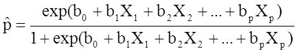 ,
,
![]() is the expected probability that the outcome is present; X1 through Xp are distinct independent variables; and b0 through bp are the regression coefficients. The multiple logistic regression model is sometimes written differently. In the following form, the outcome is the expected log of the odds that the outcome is present,
is the expected probability that the outcome is present; X1 through Xp are distinct independent variables; and b0 through bp are the regression coefficients. The multiple logistic regression model is sometimes written differently. In the following form, the outcome is the expected log of the odds that the outcome is present,
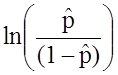 :
:
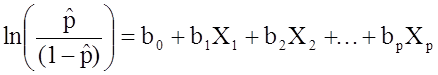 .
.
Notice that the right hand side of the equation above looks like the multiple linear regression equation. However, the technique for estimating the regression coefficients in a logistic regression model is different from that used to estimate the regression coefficients in a multiple linear regression model. In logistic regression the coefficients derived from the model (e.g., b1) indicate the change in the expected log odds relative to a one unit change in X1, holding all other predictors constant. Therefore, the antilog of an estimated regression coefficient, exp(bi), produces an odds ratio, as illustrated in the example below.
We previously analyzed data from a study designed to assess the association between obesity (defined as BMI > 30) and incident cardiovascular disease. Data were collected from participants who were between the ages of 35 and 65, and free of cardiovascular disease (CVD) at baseline. Each participant was followed for 10 years for the development of cardiovascular disease. A summary of the data can be found on page 2 of this module. The unadjusted or crude relative risk was RR = 1.78, and the unadjusted or crude odds ratio was OR =1.93. We also determined that age was a confounder, and using the Cochran-Mantel-Haenszel method, we estimated an adjusted relative risk of RRCMH =1.44 and an adjusted odds ratio of ORCMH =1.52. We will now use logistic regression analysis to assess the association between obesity and incident cardiovascular disease adjusting for age.
The logistic regression analysis reveals the following:
|
Independent Variable |
Regression Coefficient |
Chi-square |
P-value |
|
Intercept |
-2.367 |
307.38 |
0.0001 |
|
Obesity |
0.658 |
9.87 |
0.0017 |
The simple logistic regression model relates obesity to the log odds of incident CVD:
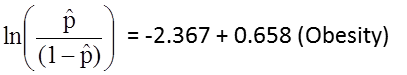
Obesity is an indicator variable in the model, coded as follows: 1=obese and 0=not obese. The log odds of incident CVD is 0.658 times higher in persons who are obese as compared to not obese. If we take the antilog of the regression coefficient, exp(0.658) = 1.93, we get the crude or unadjusted odds ratio. The odds of developing CVD are 1.93 times higher among obese persons as compared to non obese persons. The association between obesity and incident CVD is statistically significant (p=0.0017). Notice that the test statistics to assess the significance of the regression parameters in logistic regression analysis are based on chi-square statistics, as opposed to t statistics as was the case with linear regression analysis. This is because a different estimation technique, called maximum likelihood estimation, is used to estimate the regression parameters (See Hosmer and Lemeshow3 for technical details).
Many statistical computing packages also generate odds ratios as well as 95% confidence intervals for the odds ratios as part of their logistic regression analysis procedure. In this example, the estimate of the odds ratio is 1.93 and the 95% confidence interval is (1.281, 2.913).
When examining the association between obesity and CVD, we previously determined that age was a confounder.The following multiple logistic regression model estimates the association between obesity and incident CVD, adjusting for age. In the model we again consider two age groups (less than 50 years of age and 50 years of age and older). For the analysis, age group is coded as follows: 1=50 years of age and older and 0=less than 50 years of age.
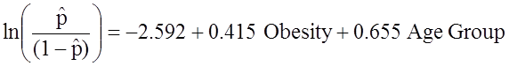
If we take the antilog of the regression coefficient associated with obesity, exp(0.415) = 1.52 we get the odds ratio adjusted for age. The odds of developing CVD are 1.52 times higher among obese persons as compared to non obese persons, adjusting for age. In Section 9.2 we used the Cochran-Mantel-Haenszel method to generate an odds ratio adjusted for age and found
![]()
This illustrates how multiple logistic regression analysis can be used to account for confounding. The models can be extended to account for several confounding variables simultaneously. Multiple logistic regression analysis can also be used to assess confounding and effect modification, and the approaches are identical to those used in multiple linear regression analysis. Multiple logistic regression analysis can also be used to examine the impact of multiple risk factors (as opposed to focusing on a single risk factor) on a dichotomous outcome.
Suppose that investigators are also concerned with adverse pregnancy outcomes including gestational diabetes, pre-eclampsia (i.e., pregnancy-induced hypertension) and pre-term labor. Recall that the study involved 832 pregnant women who provide demographic and clinical data. In the study sample, 22 (2.7%) women develop pre-eclampsia, 35 (4.2%) develop gestational diabetes and 40 (4.8%) develop pre term labor. Suppose we wish to assess whether there are differences in each of these adverse pregnancy outcomes by race/ethnicity, adjusted for maternal age. Three separate logistic regression analyses were conducted relating each outcome, considered separately, to the 3 dummy or indicators variables reflecting mothers race and mother's age, in years. The results are below.
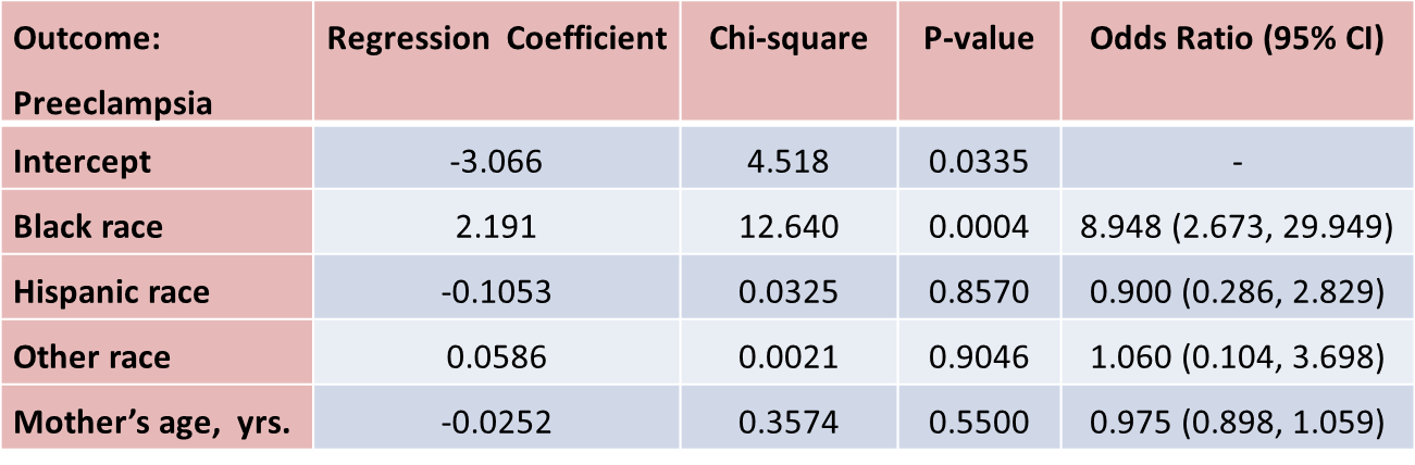
The only statistically significant difference in pre-eclampsia is between black and white mothers.
Black mothers are nearly 9 times more likely to develop pre-eclampsia than white mothers, adjusted for maternal age. The 95% confidence interval for the odds ratio comparing black versus white women who develop pre-eclampsia is very wide (2.673 to 29.949). This is due to the fact that there are a small number of outcome events (only 22 women develop pre-eclampsia in the total sample) and a small number of women of black race in the study. Thus, this association should be interpreted with caution.
While the odds ratio is statistically significant, the confidence interval suggests that the magnitude of the effect could be anywhere from a 2.6-fold increase to a 29.9-fold increase. A larger study is needed to generate a more precise estimate of effect.
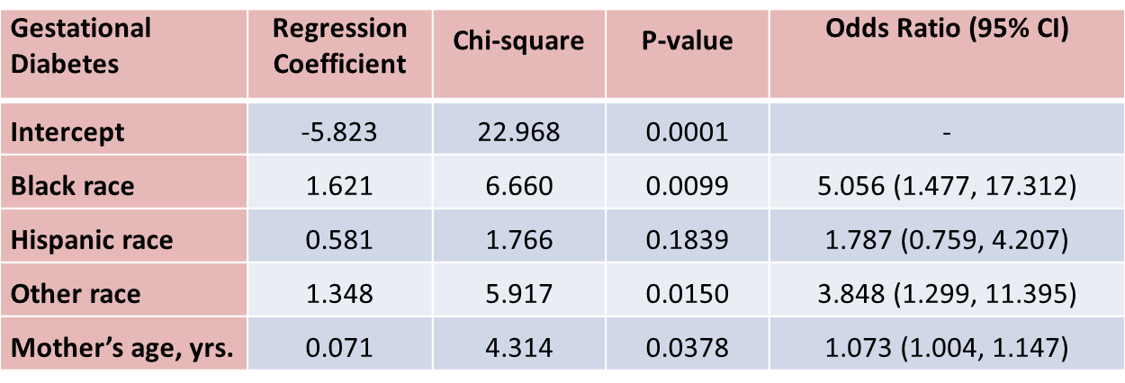
With regard to gestational diabetes, there are statistically significant differences between black and white mothers (p=0.0099) and between mothers who identify themselves as other race as compared to white (p=0.0150), adjusted for mother's age. Mother's age is also statistically significant (p=0.0378), with older women more likely to develop gestational diabetes, adjusted for race/ethnicity.
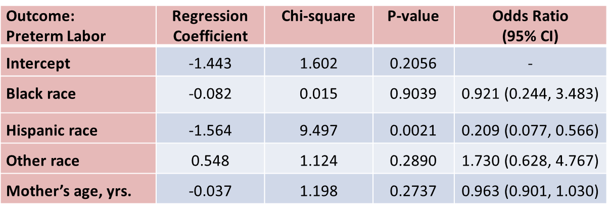
With regard to pre term labor, the only statistically significant difference is between Hispanic and white mothers (p=0.0021). Hispanic mothers are 80% less likely to develop pre term labor than white mothers (odds ratio = 0.209), adjusted for mother's age.
Multivariable methods are computationally complex and generally require the use of a statistical computing package. Multivariable methods can be used to assess and adjust for confounding, to determine whether there is effect modification, or to assess the relationships of several exposure or risk factors on an outcome simultaneously. Multivariable analyses are complex, and should always be planned to reflect biologically plausible relationships. While it is relatively easy to consider an additional variable in a multiple linear or multiple logistic regression model, only variables that are clinically meaningful should be included.
It is important to remember that multivariable models can only adjust or account for differences in confounding variables that were measured in the study. In addition, multivariable models should only be used to account for confounding when there is some overlap in the distribution of the confounder each of the risk factor groups.
Stratified analyses are very informative, but if the samples in specific strata are too small, the analyses may lack precision. In planning studies, investigators must pay careful attention to potential effect modifiers. If there is a suspicion that an association between an exposure or risk factor is different in specific groups, then the study must be designed to ensure sufficient numbers of participants in each of those groups. Sample size formulas must be used to determine the numbers of subjects required in each stratum to ensure adequate precision or power in the analysis.