


Regression Analysis
Regression analysis is a widely used technique which is useful for many applications. We introduce the technique here and expand on its uses in subsequent modules.
Simple Linear Regression
Simple linear regression is a technique that is appropriate to understand the association between one independent (or predictor) variable and one continuous dependent (or outcome) variable. For example, suppose we want to assess the association between total cholesterol (in milligrams per deciliter, mg/dL) and body mass index (BMI, measured as the ratio of weight in kilograms to height in meters2) where total cholesterol is the dependent variable, and BMI is the independent variable. In regression analysis, the dependent variable is denoted Y and the independent variable is denoted X. So, in this case, Y=total cholesterol and X=BMI.
When there is a single continuous dependent variable and a single independent variable, the analysis is called a simple linear regression analysis . This analysis assumes that there is a linear association between the two variables. (If a different relationship is hypothesized, such as a curvilinear or exponential relationship, alternative regression analyses are performed.)
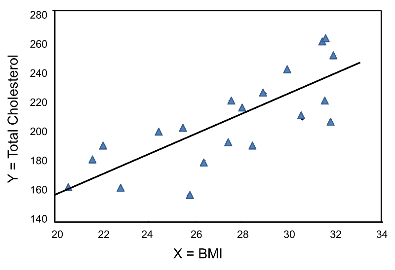
The figure below is a scatter diagram illustrating the relationship between BMI and total cholesterol. Each point represents the observed (x, y) pair, in this case, BMI and the corresponding total cholesterol measured in each participant. Note that the independent variable (BMI) is on the horizontal axis and the dependent variable (Total Serum Cholesterol) on the vertical axis.
BMI and Total Cholesterol
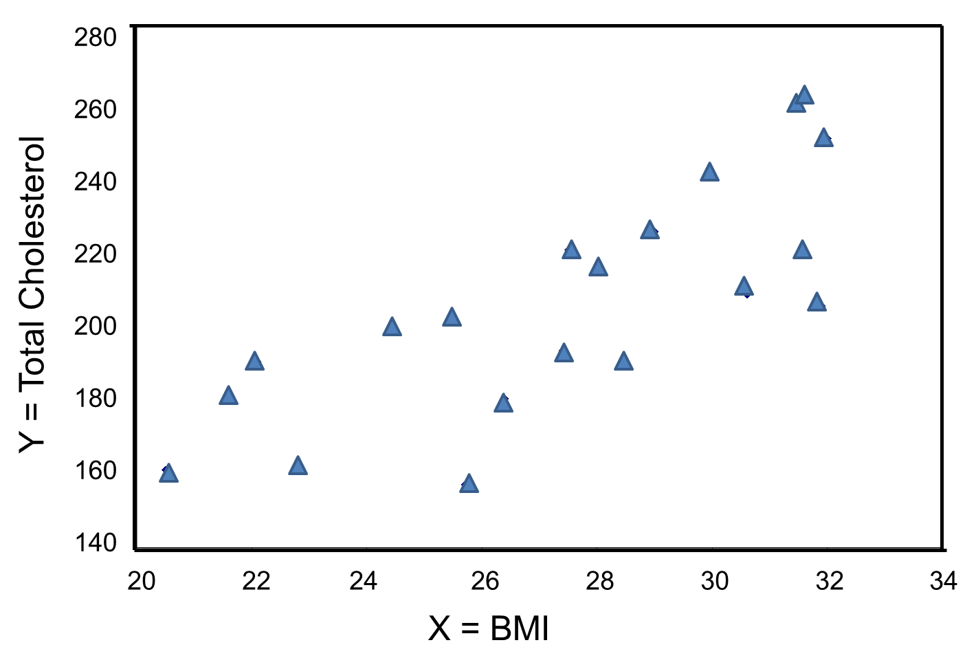
The graph shows that there is a positive or direct association between BMI and total cholesterol; participants with lower BMI are more likely to have lower total cholesterol levels and participants with higher BMI are more likely to have higher total cholesterol levels. In contrast, suppose we examine the association between BMI and HDL cholesterol.
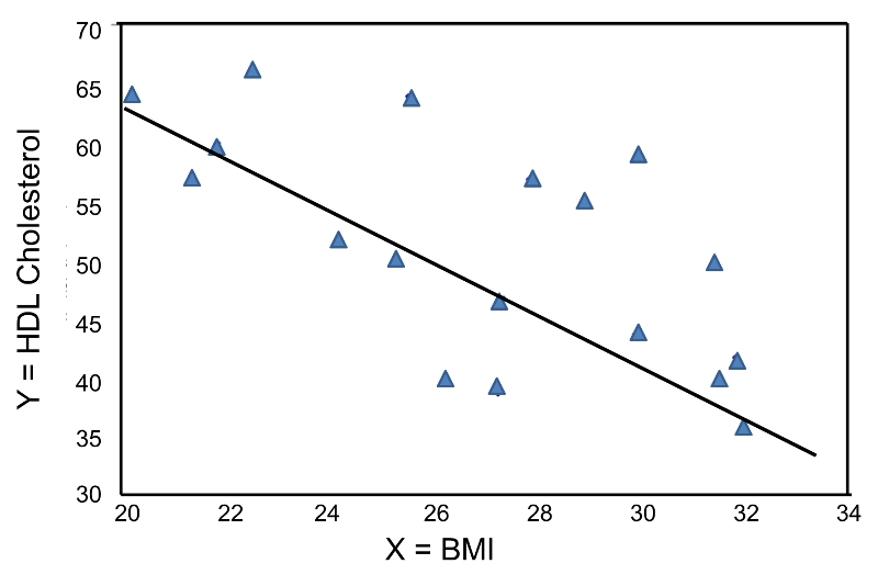
In contrast, the graph below depicts the relationship between BMI and HDL cholesterol in the same sample of n=20 participants.
BMI and HDL Cholesterol
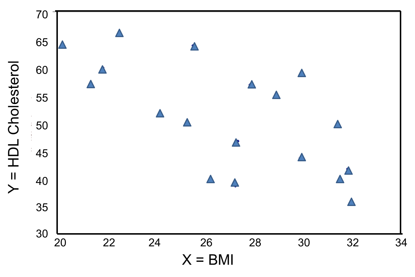
This graph shows a negative or inverse association between BMI and HDL cholesterol, i.e., those with lower BMI are more likely to have higher HDL cholesterol levels and those with higher BMI are more likely to have lower HDL cholesterol levels.
For either of these relationships we could use simple linear regression analysis to estimate the equation of the line that best describes the association between the independent variable and the dependent variable. The simple linear regression equation is as follows:


where Y is the predicted or expected value of the outcome, X is the predictor, b0 is the estimated Y-intercept, and b1 is the estimated slope. The Y-intercept and slope are estimated from the sample data, and they are the values that minimize the sum of the squared differences between the observed and the predicted values of the outcome, i.e., the estimates minimize:

These differences between observed and predicted values of the outcome are called residuals. The estimates of the Y-intercept and slope minimize the sum of the squared residuals, and are called the least squares estimates.1
|
Residuals Conceptually, if the values of X provided a perfect prediction of Y then the sum of the squared differences between observed and predicted values of Y would be 0. That would mean that variability in Y could be completely explained by differences in X. However, if the differences between observed and predicted values are not 0, then we are unable to entirely account for differences in Y based on X, then there are residual errors in the prediction. The residual error could result from inaccurate measurements of X or Y, or there could be other variables besides X that affect the value of Y.
|
Based on the observed data, the best estimate of a linear relationship will be obtained from an equation for the line that minimizes the differences between observed and predicted values of the outcome. The Y-intercept of this line is the value of the dependent variable (Y) when the independent variable (X) is zero. The slope of the line is the change in the dependent variable (Y) relative to a one unit change in the independent variable (X). The least squares estimates of the y-intercept and slope are computed as follows:

and

where
- r is the sample correlation coefficient,
- the sample means are
 and
and 
- and Sx and Sy are the standard deviations of the independent variable x and the dependent variable y, respectively.
BMI and Total Cholesterol
The least squares estimates of the regression coefficients, b 0 and b1, describing the relationship between BMI and total cholesterol are b0 = 28.07 and b1=6.49. These are computed as follows:
and

The estimate of the Y-intercept (b0 = 28.07) represents the estimated total cholesterol level when BMI is zero. Because a BMI of zero is meaningless, the Y-intercept is not informative. The estimate of the slope (b1 = 6.49) represents the change in total cholesterol relative to a one unit change in BMI. For example, if we compare two participants whose BMIs differ by 1 unit, we would expect their total cholesterols to differ by approximately 6.49 units (with the person with the higher BMI having the higher total cholesterol).
The equation of the regression line is as follows:
The graph below shows the estimated regression line superimposed on the scatter diagram.
The regression equation can be used to estimate a participant's total cholesterol as a function of his/her BMI. For example, suppose a participant has a BMI of 25. We would estimate their total cholesterol to be 28.07 + 6.49(25) = 190.32. The equation can also be used to estimate total cholesterol for other values of BMI. However, the equation should only be used to estimate cholesterol levels for persons whose BMIs are in the range of the data used to generate the regression equation. In our sample, BMI ranges from 20 to 32, thus the equation should only be used to generate estimates of total cholesterol for persons with BMI in that range.
There are statistical tests that can be performed to assess whether the estimated regression coefficients (b0 and b1) are statistically significantly different from zero. The test of most interest is usually H0: b1=0 versus H1: b1≠0, where b1 is the population slope. If the population slope is significantly different from zero, we conclude that there is a statistically significant association between the independent and dependent variables.
BMI and HDL Cholesterol
The least squares estimates of the regression coefficients, b0 and b1, describing the relationship between BMI and HDL cholesterol are as follows: b0 = 111.77 and b1 = -2.35. These are computed as follows:
and

Again, the Y-intercept in uninformative because a BMI of zero is meaningless. The estimate of the slope (b1 = -2.35) represents the change in HDL cholesterol relative to a one unit change in BMI. If we compare two participants whose BMIs differ by 1 unit, we would expect their HDL cholesterols to differ by approximately 2.35 units (with the person with the higher BMI having the lower HDL cholesterol. The figure below shows the regression line superimposed on the scatter diagram for BMI and HDL cholesterol.
Linear regression analysis rests on the assumption that the dependent variable is continuous and that the distribution of the dependent variable (Y) at each value of the independent variable (X) is approximately normally distributed. Note, however, that the independent variable can be continuous (e.g., BMI) or can be dichotomous (see below).