


Authors:
Lisa Sullivan, Professor of Biostatistics
Wayne W. LaMorte, MD, PhD, MPH, Professor of Epidemiology
Boston University School of Public Health
Simple Linear Regression
Regression analysis makes use of mathematical models to describe relationships. For example, suppose that height was the only determinant of body weight. If we were to plot height (the independent or 'predictor' variable) as a function of body weight (the dependent or 'outcome' variable), we might see a very linear relationship, as illustrated below.

We could also describe this relationship with the equation for a line, Y = a + b(x), where 'a' is the Y-intercept and 'b' is the slope of the line. We could use the equation to predict weight if we knew an individual's height. In this example, if an individual was 70 inches tall, we would predict his weight to be:
Weight = 80 + 2 x (70) = 220 lbs.
In this simple linear regression, we are examining the impact of one independent variable on the outcome. If height were the only determinant of body weight, we would expect that the points for individual subjects would lie close to the line. However, if there were other factors (independent variables) that influenced body weight besides height (e.g., age, calorie intake, and exercise level), we might expect that the points for individual subjects would be more loosely scattered around the line, since we are only taking height into account.


Multiple Linear Regression Analysis
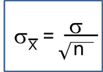
Multiple linear regression analysis is an extension of simple linear regression analysis which enables us to assess the association between two or more independent variables and a single continuous dependent variable.
![]()
![]()
This is a very useful procedure for identifying and adjusting for confounding. To provide an intuitive understanding of how multiple linear regression does this, consider the following hypothetical example.
Suppose an investigator had developed a scoring system that enabled her to predict an individual's body mass index (BMI) based on information about what they ate and how much. The investigator wanted to test this new "diet score" to determine how closely it was associated with actual measurements of BMI. Information is collected from a small sample of subjects in order to compute their "diet score," and the weight and height of each subject is measured in order to compute their BMI. The graph below shows the relationship between the new "diet score" and BMI, and it suggests that the "diet score" is not a very good predictor, (i.e., there is little if any association between the two.

While this is discouraging, the investigator considers that it is possible that confounding by age and/or gender is masking the true relationship between "diet score" and BMI. She first identifies which subjects who are older than 20 years old, and it turns out that the younger subjects and older subjects are clustered in the scatter plot, as shown in the figure below.

The investigator suspected that gender might also be a confounding factor, and when she identified males and females, the graph looked like this:
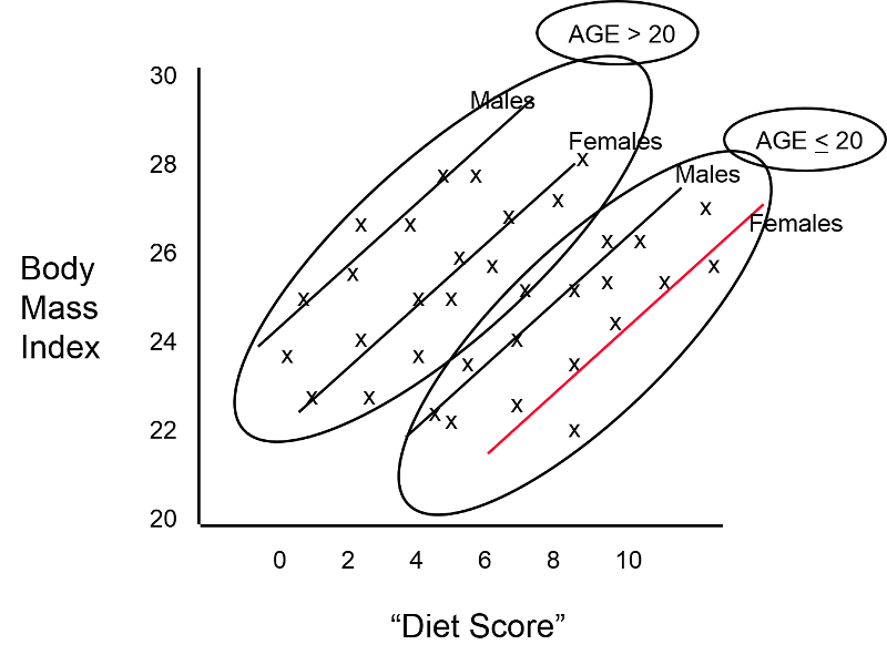
These findings indicate that both age and gender have an impact on BMI, because the older group has higher BMIs than the younger group, while males consistently have higher BMIs than the females. In addition, age and gender are also associated with "diet score," which is the "exposure" of interest, because diet scores are not equally distributed by gender or by age. In other words, both age and gender meet the criteria to be confounders. We can also see (in this very hypothetical example) that there is a striking linear relationship between "diet score" and BMI within each of the four age and gender groups. In other words, it is only after "taking into account" these two confounding variables that we can see that there really is a relationship between diet score and BMI. The true relationship was confounded by these other factors.
When analyzing data, it is always easier to deal with numeric data instead of text. For example, when dealing with dichotomous data the number "1" might conveniently indicate that the characteristic is present instead of "yes" or "true," and the number "0" conveniently indicates "no" or "false". It is also best to organize data sets so that the information for individual subjects is listed in a row, and the columns contain the variables. Consequently, in this scenario my data set would perhaps look something like this:
|
Subject ID |
Diet Score |
Male |
Age>20 |
BMI |
|---|---|---|---|---|
|
A |
4 |
0 |
1 |
27 |
|
B |
7 |
1 |
1 |
29 |
|
C |
6 |
1 |
0 |
23 |
|
D |
2 |
0 |
0 |
20 |
|
E |
3 |
0 |
1 |
21 |
|
etc. |
... |
... |
... |
... |
With data is are coded in this fashion, matrix math can be used to find the coefficients for each variable that led to the best "fit" of the data. For the hypothetical example we are considering here, multiple linear regression analysis could be used to compute the coefficients, and these could be used to describe the relationships in the graph mathematically with the following equation:
BMI = 18.0 + 1.5 (diet score) + 1.6 (male) + 4.2 (age>20)
Note that the numbers in red are the coefficients that the analysis provided.
The Independent Effect of Each Independent Variable
In a sense, the equation above is a prediction of what an individual's BMI will be based on their diet score, gender and age group. The equation has an intercept of 18.0, meaning that I start with a baseline value of 18. I then multiply 1.5 x (diet score); I multiply 1.6 x (male) and multiply 4.2 x (age>20). But remember that in the data base I coded male as 1 for males and as 0 for females; for age group I coded it as 1 if the subject was older than 20 and coded it as 0 if they were less than 20.
Besides being useful for describing the relationships and making predictions, this mathematical description provides a powerful mean of controlling for confounding. For example, the coefficient 1.5 for diet score indicates that for each additional point in diet score, I must add 1.5 units to my prediction, regardless of whether it is a male or female or an adult or a child. In other words, the equation has quantified the association of diet score on BMI independent of (i.e., controlling for) gender and age group. Similarly, it means that I should add 1.6 units to my prediction if the individual is a male, regardless of there age and diet score. And I should add 4.2 to my prediction if the person is over age 20, regardless of their diet score or gender. As a result, the regression analysis has enabled us to dissect out the independent (unconfounded) association of each factor with the outcome of interest. The equation describes the graphical representation of this data, shown below.
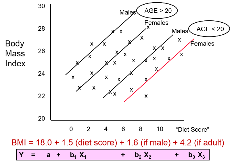
The figure above and the equation enable us to see the impact of each of the independent variables after controlling for confounding. The equation is a mathematical expression of what we see in the figure, and the coefficients for each variable describe an unconfounded measure of the association of each variable with the outcome.