Exposure Assessments
Introduction to Basic Concepts
From the water we drink, swim or bathe in, the air we breathe, to the consumer products we apply in/on our bodies and our surrounding environments, to the soil we use to grow our food, we are exposed to environmental agents in every aspect of human life and activity. Exposure assessment is a branch of environmental science that attempts to characterize how these contaminants behave in the environment and subsequently result in human exposure. The goal of an exposure assessment applied in the traditional environmental health context is to quantitatively measure how much of an agent can be absorbed by an exposed population, in what form are they exposed, at what rate is exposure occurring, and how much of the absorbed amount is actually available to produce a biological effect
This module is intended to provide an introductory overview to exposure assessments. This module offers a basic understanding of the steps and key considerations involved in designing and conducting an exposure assessment, mainly in the context of epidemiological studies.
After completing this module, users will be able to:
According to the EPA, an exposure assessment is the "process of measuring or estimating the magnitude, frequency, and duration of human exposure to an agent in the environment, or estimating future exposures for an agent that has not yet been released." Exposure assessments attempt to address some of the following questions.
Exposure assessments are generally used to characterize occupational exposures in the workplace and environmental exposures to the general population, such as emissions from industrial processes, contaminated food or water, consumer products containing hazardous chemicals, etc. The table below highlights the different applications for an exposure assessment.
|
Applications for an Exposure Assessment |
|
|
Epidemiological study |
In an epidemiological study, investigators are assessing whether exposure to an environmental contaminant or agent is associated with a given health outcome. The goal is ultimately to determine if a causal relationship takes place between exposure and disease. |
|
Occupational health |
Occupational health studies often attempt to characterize exposure and risk of exposure in the context of work-related activities. The goal is to both identify and control risks that result from physical, chemical, and other workplace hazards. |
|
Risk assessment |
With the goal of a risk assessment being to characterize the nature and magnitude of health risks from chemical contaminants and other stressors, the exposure assessment is the component that attempts to characterize who is exposed and how much are they exposed to. |
|
Routine surveillance
|
Routine surveillance may be required by various types of industry to determine whether they meet regulatory standards put forth by agencies such as the EPA and OSHA. For example, the EPA's Great Lakes Fish Monitoring and Surveillance Program collects fish from the Great Lakes annually and analyzes them for contaminants. |
|
Other |
Other applications for exposure assessments include evaluating the effectiveness of an intervention strategy. |
Exposure is referring to when individuals come into contact with a substance or factor affecting human health, either adversely or beneficially. According to IUPAC glossary, exposure is defined as the "concentration, amount or intensity of a particular physical or chemical agent or environmental agent that reaches the target population, organism, organ, tissue or cell, usually expressed in numerical terms of concentration, duration, and frequency (for chemical agents and micro-organisms) or intensity (for physical agents)." Although this definition mentions contact with internal components of the body, exposure takes place externally on the body and does not automatically lead to an internal dose. There is a distinction between the external dose one is exposed to and the internal dose that is absorbed since they are not always the same. The units used to express exposure are concentration times time.
In order for exposure to occur, an individual has to be exposed to an agent. Identifying and understanding the behavior of the causal agent is paramount to understanding how an individual became exposed and any subsequent health effects. The physical and chemical properties of an agent will influence how it behaves in the environment (fate and transport) as well as in tissues (absorption, distribution, metabolism, and excretion).
While the methods involved in any given exposure assessment will vary depending on the specific objective(s) of the study, the principles and basic components of an exposure assessment remain the same. The activity below highlights some important factors involved in conducting an exposure assessment. While these considerations will be explained in greater detail throughout the module, you may scroll over each item below for a brief overview.
The steps involved in being exposed to a contaminant of concern to a resulting adverse health outcome must be explored and established when conducting an exposure assessment. This involves identifying sources of exposure, how the contaminant behaves in the environment, and the context in which people come into contact with the contaminant that results in an adverse health effect. Below is a conceptual model for exposure-related disease that can be helpful in understanding the pathway from exposure to disease.
The exposure pathway is the physical course an environmental agent takes from its source to the receptor. To characterize the exposure pathway, one must consider the fate and transport of a given agent, meaning how will it behave in the environment or media and how or if it will come into contact with humans. If an agent is produced and emitted from a stack into the air, it will be available to the surrounding community in the ambient air, probably in the direction of the prevailing winds. If the agent is discharged into a river, then it will be available to the water and the biota in the river. The biota may be able to chemically change the agent so that when a person eats the biota, the agent may be more or less toxic than when it was originally discharged into the river.
Another factor that must be considered regarding a chemical's fate and transport is its potential for degradation in the environment and its half-life in specific environmental media. Some chemicals are broken down rapidly by sunlight, water, or bacteria into less toxic forms, while others may remain in the same form for a long time. Alternatively, some chemicals may form even more toxic by-products when they decay. The term used to describe a chemical that is resistant to degradation is "persistent." Persistent organic pollutants, such as. In addition, many chemicals bioaccumulate in the environment. For example, PCBs concentrate in fish and birds that eat fish.
The routes of exposure are the pathways by which humans are exposed to agents. Agents of concern may have different toxicities depending on the routes of exposure. Inhalation, ingestion, and dermal contact are typically the exposure routes for environment contaminants.
For example, one might be exposed to intact lead paint on a windowsill by touching it. In this manner, the lead is not harmful. However, should the windowsill be sanded, you are now exposed to the lead by inhaling it, making it toxic as a function of the route of exposure.
Often times the agent of concern can be directly measured or modeled at the point of contact, for example, in the breathing zone, on the skin, or via dietary assessments.
Understanding the media in which an agent is found will allow you to understand the ways in which humans may be impacted. Some common media are:
Being able to understand and effectively evaluate journal articles is an important skill. The tabbed activity below highlights some important considerations for evaluating an exposure assessment. Note that some of the concepts mentioned in the activity will be described in greater detail throughout the module. A hard copy version of the activity can be access in the "More Resources" menu on the right.
Exposure assessments can be applied in many different contexts meaning the objectives can be very different from one study to the next. In occupational and environmental epidemiology, investigators are often attempting to examine the relationship between an exposure and a health outcome of interest. Examples of common study designs used in occupational and environmental epidemiology include case-control, cohort, cross-sectional, and time series. For more information on epidemiological study designs, review the following modules: descriptive epidemiology and overview of analytical epidemiology.
When designing a study to estimate exposure, it is important to take into consideration the following questions:
It is important to distinguish between what the actual agent of concern is and what is being measured in the study. At times it may be difficult or impossible to measure exposure to the actual agent. In such cases, exposure to a surrogate is estimated. The surrogate being used to measure exposure should closely correlate with the actual causal agent. Another important consideration when using surrogates is identifying where they belong on the exposure-response pathway.
While investigators can measure exposure at the source or in the media, such measurements may not accurately reflect actual exposure due to factors such as the environmental fate and transport of a given agent. Biomarkers are an example of a surrogate that is more indicative of the absorbed dose of a given agent as opposed to the actual exposure for an individual or population. Factors such as absorption, distribution, metabolism, and excretion will affect how much of the exposed agent is bioavailable.
Exposure assessments are often tasked with trying to obtain accurate, precise, and biologically relevant exposure estimates in the most efficient and cost-effective way. The data collection methods employed by an exposure assessment often require a balancing act between accuracy/precision of data and logistic constraints, such as time, money, and resources. If too much of the accuracy and precision are compromised during this balancing act, errors such as misclassification of exposure can be introduced into the study resulting in attenuated estimates and even loss of power. Such error will be discussed later in the module.
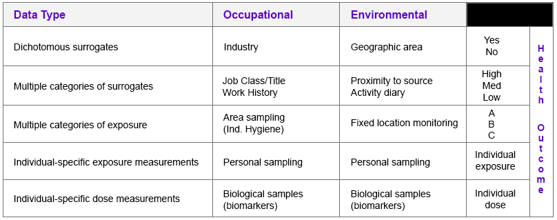
Exposure can be classified, measured, or modelled with what are often referred to as direct or indirect methods.
Classification: Subjects in an exposure assessment can be classified using dichotomous values such as "exposed" or "not exposed" to a particular substance. Classifications can also incorporate multiple categories of exposure, such as "no", "low", "medium", and "high" or different job titles for an occupational study. Such classifications can be obtained through questionnaires or by expert assessment.
Measurement: As a direct method, measurements are often considered a more objective means of assessing exposure. The most common measurement utilized is the concentration of a given agent. Area monitors are used to estimate exposure to individuals living within a certain proximity and personal monitors can be used to measure individual-specific exposure.
Modelling: Modelling of exposure is often carried out in conjunction with measurements and can be helpful when there is a lack of monitoring data. Exposure assessment models are often based on assumptions about actual exposure and more sophisticated models will takes into consideration factors that may influence exposure (e.g. physical and chemical properties, and fate and transport of an agent). Sources such as the EPA provide a variety of models that can be utilized by researchers to predict exposure.
Shown below is a diagram that provides some examples of collecting exposure data and the different methods that can be employed.
The number of samples collected, the number of subjects in the study, and the number of locations from which samples are collected are all important considerations that directly affect the statistical power of any study performed. Determining sample size is often an issue of trying to overcome random error. Sample size calculations are often performed to determine how many samples or subjects are required to detect a statistically significant difference between the population mean hypothesized under the null and alternative hypotheses. To learn more, you may review the modules on sample size and power and random error.
Environmental exposures present some unique challenges investigators must consider with respect to sample size. Both sample size and magnitude of effect can influence statistical power. Environmental exposures are common and relatively low making it difficult to find unexposed groups and the magnitude of effect small. In order to offset these factors that can diminish the statistical power of a study, larger sample sizes are required.
Hypothesis testing can lead to type I & II errors which are described in the interactive diagram below. Small sample size is a common reason for type II errors.
|
Type I & II Error Explained with a Fable
The boy who cried wolf is a well known fable that can help explain type I and type II errors.
|
When conducting an exposure assessment and designing a study, the consequences of having a poorly defined population can be costly and undermine the validity of the study. In evaluating the effect of an agent, investigators must consider the media that are contaminated and whether people in the community are exposed to that media, meaning they are drinking that water, breathing that air, eating those biota, or having skin contact with those soils or other media. Also, consider the presence and location of microenvironments, such as schools, nursing homes, hospitals, daycare centers, etc.
It is important to consider special populations that may have increased susceptibility to adverse effects upon exposure to a given agent. Examples of special populations that may be particularly vulnerable or sensitive to the effects of certain agents include children, people with chronic illnesses, pregnant women and their fetuses, nursing women, and the elderly.
There are three dimensions to exposure: duration, concentration, and frequency. Given the dimensions of duration and frequency, it becomes clear that time plays a key role in estimating exposure. One must consider a relevant time period in relation to the outcome. Depending on how long exposure has occurred, the health outcomes may vary. Long-term, chronic exposure to a given agent will often result in different outcomes compared to short-term, chronic exposures.
The duration of exposure may also affect which study design is chosen. In the case of long-term exposures, a retrospective cohort (in which exposure has already occurred) or cross-sectional study might be more feasible. Longitudinal studies in which subjects are followed for a period of time until the development of a given outcome tend to yield more internal validity, but also prove to be more costly and require a greater amount of resources.
In the event that exposure is being monitored, investigators must determine a sample duration time to collect exposure information. For example, investigators in an occupational exposure assessment may use a work shift as the sampling duration.
All exposure assessments require some way of measuring exposure to a given agent, which can result in measurement error (i.e. exposure measurements determined from samples are not representative of actual exposure). Measurement error is the difference between the true exposure and a measured or observed exposure. While large inter-individual or inter-group differences can be important to detect statistically significant differences, investigators do not want such large inter-individual differences among individuals with similar exposures (i.e. between-subject variability).
Common sources of measurement error include the following:
The table below uses a regression equation to demonstrate the impact measurement error can have on risk estimates in a given study. The first equation highlights what investigators want which is being able to determine the health outcome ("y") based on true exposure ("x"). However, investigators determine health outcome as a function of a measured/observed exposure ("z"). The key concern is the difference between βx and βz.
|
Impact on Risk Estimates |
|
|
What investigators want: y = α + βxx + ε What investigators have: yij = α + βzzij + εij
|
The two types of error that can result from measurements are systematic and random error, which can affect the accuracy and precision of exposure measurements. Suppose investigators wanted to monitor changes in body weight over time among the students at Boston University. In theory, they could weigh all of the students with an accurate scale, and would likely find that body weight measurements were more or less symmetrically distributed along a bell-shaped curve. Knowing all of their weights, investigators could also compute the true mean of this student population. However, it really isn't feasible to collect weight measurements for every student at BU. If investigators just want to follow trends, an alternative is to estimate the mean weight of the population by taking a sample of students each year. In order to collect these measurements, investigators use two bathroom scales. It turns out that one of them has been calibrated and is very accurate, but the other has not been calibrated, and it consistently overestimates body weight by about ten pounds.
Now consider four possible scenarios as investigators try to estimate the mean body weight by taking samples. In each of the four panels (shown below), the distribution of the total population (if investigators measured it) is shown by the black bell-shaped curve, and the vertical red line indicates the true mean of the population. Review the illustration below for more information.
For environmental exposures, exposure data is often collected on an aggregate scale since individual exposure measurements can be difficult or impossible to collect, which can lead to random misclassification of exposure. Another source of random misclassification takes place as a result of the intra-individual (within-subject) variability, particularly when investigating chronic effects. For example, a study looking to assess dietary pesticide exposure may need to address how dietary intake for an individual may change seasonally, which would result in different exposure levels for the same individual.
Non-random, or differential misclassification of exposure takes place when errors in exposure are more likely to occur in one of the groups being compared. Random misclassification of exposure is when errors in exposure are equally likely to occur in all exposure groups. Random misclassification can be broken down into two categories: Berkson error model and classical error. Berkson error model refers to random misclassification that results in little to no bias in the measurement whereas classical error refers to random misclassification that tends to attenuate the risk estimates (i.e. bias towards the null).
There are measures that can be taken throughout a study (design, data collection, and analysis phase) to minimize or adjust for measurement error. For example, validation studies are studies that attempt to assess a given method of collecting exposure compared to a "gold standard." For example, a study might collect a single urine sample from study participants to analyze it for organophosphate metabolites. But the "gold standard" is to collect 24-hour urine samples. A validation study attempts to determine the level of agreement between the single urine sample and 24-hour urine samples.
Data analysis is the means through which investigators can communicate valuable information about the exposure-disease pathway. In other words, what is there an association between the exposure of interest and the health outcome of interest? If so, what is the nature of this relationship? While statistical numbers and visual displays are an important component of the data analysis, there are other aspects. When thinking about data analysis, the items below provide a more comprehensive look at data analysis.
Maintaining the integrity of data collected and having a protocol for how that data will be coded and analyzed is essential to any exposure assessment. A data management plan is a formal document developed by investigators in the design phase of a study that describes how investigators will handle the data during and after the study. There are three key stages that can be considered integral to any data management plan: preparatory, data organization, and the analysis and dissemination.
Think about the multiple steps involved in measuring an exposure of interest. With the use of measuring equipment, a process is employed to set up in the "field" often followed by some sort of transport from the field to a lab or some other location in order to extract and analyze information about the exposure. There are many opportunities for contamination to occur that can affect the results of the exposure data. In order to minimize errors that may be introduced in the exposure collection process, there are several methods that can be incorporated into the study protocol.
According to the EPA, the "primary purpose of blanks is to trace sources of artificially introduced contamination." In addition to blanks, investigators can utilize different sampling methods to assess and correct for measurement error introduced during the data collection and sampling analysis process. Review the activity below for definitions and examples of these quality assurance/quality control measures.
The processes involved in collecting, preparing, and analyzing sample concentrations can yield measurements that are different from the true sample value as a result of contamination or errors with the sampling method. Sample values must be evaluated and possibly corrected for contamination, accuracy, and precision. Corrected sample concentrations represent the "true" sample level without any effects from sample preparation, analysis, or collection
Analytical instruments and techniques can produce a signal even when analyzing a blank, which is why a limit of detection must be established. The limit of detection, or detection limit, is the smallest amount of a substance that can be determined to be significantly different from background noise or a blank sample. There are several different detection limits that are commonly used. The list below highlights detection limits based on the instrument used to analyze the substance or the overall method.
|
Common approaches for analyzing results below the detection limit:
|
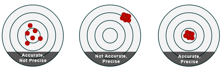
By assessing accuracy, we address the question: what is the "true value" relative to the sample value? The goal is to account for any measurement error that may affect the sample value by causing it to deviate from the true value. When assessing precision, the question becomes: how much variability exists among the sample values? The image below illustrates different scenarios of accuracy and precision with the bulls eye representing the "true value" or "true exposure."
There are several methods that can be employed in order to assess the level of accuracy and precision in a study. Examples are provided in the diagram below.
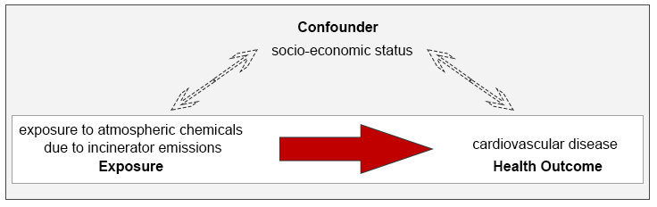
For studies assessing the relationship between exposure and an outcome, confounding and effect modification are two factors that can affect the results of the study by over- or underestimating the true magnitude of the effect. Confounding occurs when variables other than the exposure might explain the relationship seen between incinerators and poor health outcomes. The illustration below highlights a scenario in which investigators wish to assess the relationship between incinerator emissions and cardiovascular disease. In this case, socio-economic status (SES) can be a confounding factor since it is associated with both the exposure and the health outcome independently.
Effect measure modification is when the magnitude of effect seen between an exposure and health outcome is somehow modified by a third variable. Some medications are known to be more effective in men compared to women, making sex an effect modifier in such cases. A study looking at the effects of fluoride exposure and hip fractures should consider the fact that elderly women are at increased risk of hip fractures when compared to men. To learn more about how to address confounding and effect modification in a study, you may review the module on confounding & effect modification.
The table below highlights some measures for minimizing and controlling for confounding. Note that effect modifiers can only be reported and cannot be adjusted via analytical techniques.
|
Minimizing and Controlling for Confounding |
|
Study Design
Analysis Phase Analytical techniques can be utilized to adjust for confounding given investigators have collected information on the confounder such as by collecting baseline characteristics.
|
When it comes to the findings of an exposure assessment, numbers alone often do not tell the whole story since valuable information such as trends (e.g. dose-response relationships) often require some visual representation. Investigators must identify the most meaningful way to communicate the story being told by the data. One of the key considerations when presenting data is to ensure that specific objectives and aims have been identified (the design portion of the study) and that any analyses performed addresses those objectives.
The following are some common ways data may be evaluated and subsequently presented in exposure assessments. For more information, you may view a module on data presentation.
While some exposure assessments collect surrogate data such as job titles, work history, questionnaire data, other studies use more direct methods such as measurement data through monitoring of the exposure. Measurement data is commonly collected in the form of a concentration of the agent of interest. Such methods are generally seen as more objective and can consist of area or personal monitoring. Given the amount of resources required to carry out personal monitoring, this can often be a less feasible choice for collecting exposure data.
The remainder of the module will introduce some of the basic concepts for air, biological, dermal, dietary, and noise monitoring, including examples of monitoring methods, equipment, limitations and considerations.

In order to perform air sampling methods, investigators must consider the phase of the pollutant of interest, the sample type and sample duration. There are two basic categories involved with air sampling: gases/vapors and particulate matter. Highlighted below are some distinguishing properties of the different categories.
Gases & Vapors: Gases occupy the entire space of their enclosure and do not exist in a liquid state at STP. Examples include nitrous oxide, ozone, and carbon monoxide. Vapors are the evaporation products of compounds that may exist in a liquid state at STP. Vapors may condense at high concentrations and coexist in both gas and aerosol forms. Examples include toluene, benzene, and mercury.
Particulate matter (PM): PM refers to either solid particles or liquid droplets suspended in gas. Aerosol refers to the particulate and gas together. The following are examples of particulate matter: dusts, mists, fumes, smoke and fibers. Knowing the chemical composition of particulate matter is crucial in order to understand the possible health effects. The size of PM also determines the extent of exposure since the smallest particles can actually reach the bloodstream while larger particles cannot get past the upper airway.
|
Basic Calculations for Air Monitoring |
|
Calculating Concentration: Measurements for particulate matter, gases, and vapors are often expressed as the mass of contaminant per cubic meter of air, ug/m3 or mg/m3. Example: An IH samples for cobalt dust at 2 liters/minute (lpm) for 7 hours and after laboratory analysis finds that 0.11 mg of cobalt has been collected. If we wanted to calculate the average concentration of cobalt dust in the air during the 7 hours, we would use the following calculation: 2 L/min x 7hr x 60 min/1 hr = 840 liters of air samples 0.11mg Cobalt/840 liters air x 1000 liters/1 m3 = 0.13 mg/m3 Converting mg/m3 to ppm: When measuring vapors or gases, measurements can be expressed as mg/m3 or parts per million (ppm) or parts per billion (ppb). Below is the formula to convert mg/m3 to ppm where "MW" stands for molecular weight of the agent. This formula can be used when measurements are taken at 25*C and 1 atmosphere. parts per million (ppm) = (mg/m3 x 24.45)/ MW Time-Weighted Average: Time-weighted average is generally used in occupational health as a measure of workers daily exposure to a hazardous substance and is averaged to an 8-hour workday, taking into account the average levels of the agent and the time spent in the area. A time-weighted average is equal to the sum of the portion of each time period (as a decimal, such as 0.25 hour) multiplied by the levels of the substance or agent during the time period divided by the hours in the workday (usually 8 hours). Below is the calculation where C1 is the concentration during T1 and Ttotal is total time. Time-Weighted Average (TWA) = (C1T1 + C2T2 + C3T3...CnTn)/Ttotal |
How the pollutant of interest follows along the exposure-disease pathway (from source to health outcome) will greatly influence the sampling method chosen. Resources and feasibility also play an important role. Highlighted below are three broad categories of sampling methods.
The duration of sampling may depend on several factors including study feasibility and the nature of the contaminant source. Investigators must strike a balance between the need to collect samples that are reasonably representative of the desired exposure and the constraints resulting from limited finances and resources.
With a relatively constant source, the assumption is that the emission rate and ultimate concentration does not fluctuate. This generally allows for sampling durations of shorter duration thus a shorter duration time (i.e., several hours of sampling) would be representative of a 24-hour period.
With sources that result in more variation (e.g. emissions from an industrial plant tend to vary depending on hours of operation), longer durations of sampling may be necessary to capture more representative data. Sampling durations can include the use of minimum and maximum sampling volumes, minutes, hours, work-shifts, representative timeframes, and 24 hours.
|
Resources for sampling and analytical methods
|
The following table provides examples of the different types of sampling equipment that can be used to collect air monitoring data. Note this is not a comprehensive list of air sampling equipment and is designed to provide an overview of some of the mechanisms behind air sampling equipment and how they collect air samples.
|
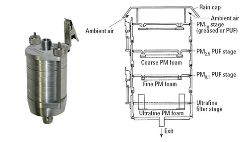
Active Sampling of PM There are several methods available for actively sampling particulate matter. Size-selective sampling is the collection of one particle size fraction, such as the collection of PM10 or PM2.5. If the objective is to obtain data regarding a particular PM size, cyclones and single stage impactors can be used to remove large particles from the sample followed by a filter for aerosol collection. Size-segregated sampling refers to the physical separation of airborne particles into several size fractions, which can be achieved with the use of cascade impactors (right) and virtual impactors. Shown in Figure 1 is a cascade impactor with its schematic illustrating how it collects particles of different sizes on separate plates.
|
Figure 1 |
|
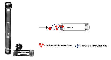
Active Sampling of Gases/Vapors A sampling pump is required to actively sample gases and vapors. One method involves the use of sorbent tubes, which contain collection materials such as activated charcoal, silica gel, tenex, etc. Another method involves the use of annular denuders shown in Figure 2 in which the agent of interest is adsorbed onto the wall coated with suitable collection material. The particles and undesired gases will pass through while the target gases will removed adsorbed onto the wall. While this method still requires a pump, it also relies on diffusion to collect the gas or vapors.
|
Figure 2 |
|
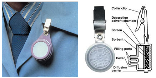
Passive Sampling of Gases/Vapors Passive sampling does not require a pump. Passive samplers have been developed for many gaseous pollutants (e.g. NO2, O3, VOCs, etc.). The sampling rate is controlled by a physical process, such as diffusion through a static air layer or permeation through a membrane. It's important to note that factors such as temperature, high humidity, and face velocity can affect the sampling process. Shown in Figure 3 is a vapor diffusion badge that can be used to passively sample vapors. It's relatively easy to use and there are many types (contaminant-specific) available.
|
Figure 3 |
The article below by Dadvand et all investigates the relationship between surrounding greenness and personal exposure to air pollution among pregnant women. Note in this study, the health outcome investigators set to evaluate is reduced disease or a "protective" effect. Review the introduction and study methods prior to answering the questions below the article.

|
Image Citations
|
Skin is considered to be the largest organ and serves many functions. On the one hand, skin serves as a protective barrier from the external environment (physical, chemical, and biological barrier). Skin also plays an important role in absorption by allowing some substances to pass through the skin and into the bloodstream. While some substances such as vitamins from the sun play an important role in maintaining health, harmful substances can also be absorbed through skin.
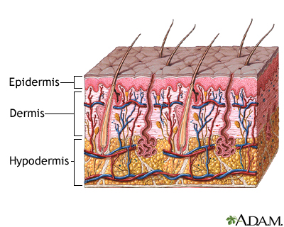
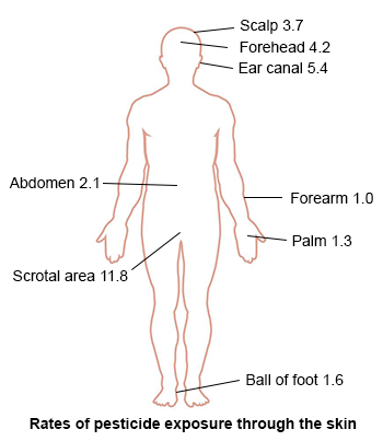
As shown in the image below on the left, there are three main layers that make up the skin: the epidermis, the dermis, and the hypodermis. The stratum corneum is the outermost portion of the epidermis and consists of dead cells, which are replaced every 2-3 weeks. The make up of this layer is such that it functions to protect underlying tissues from dehydration as well as chemicals and mechanical stress. It acts as a rate-limiting diffusion barrier. The image on the right highlights how different parts of the body can absorb chemicals such as pesticides through the skin at different rates. Note the areas that have the highest rate compared to the lowest rate.
|
|
|
Understanding the dynamics of how chemicals can be absorbed through the skin reveals some important factors that influence skin absorption. Chemicals penetrate the skin through passive diffusion, meaning a transfer of a given chemical through the skin occurs when there is a concentration gradients. Steady-state rate of transfer across a homogeneous membrane is determined by Fick's first law of diffusion shown in the table below.
|
Fick's First Law of Diffusion |
|
|
Jss = KmvD/l ΔC
|
Experimental results are frequently summarized as a permeability coefficient Kp (cm/hr), which is used to calculate absorbed dermal dose rates in a given scenario. Kp values are chemical-specific and are essential for characterizing transport through skin and are often calculated as a function of Kow and molecular weight. The EPA uses the following formula to calculate the Kp.
|
Skin Permeability Coefficient (Kp) |
|
|
log Kp = 0.71 * log Kow - 0.0061 * MW - 2.72
|
|
|
** It's important to note that the relationship expressed in this formula does not hold well for small polar molecular weight compounds or for large lipophilic compounds. |
There are three general categories of dermal exposure assessment methods highlighted below. All of the following methods measure mass of material on the skin surface, though each measures slightly different aspects of dermal exposure.
|
Fluorescent tracer techniques Fluorescent tracer techniques rely on the measurement of UV fluorescence from materials deposited and retained on the skin. This method is often used to mimic pesticide exposure in which a fluorescent tracer is mixed, diluted, and applied like pesticides. Then a blacklight is used to reveal the patterns and areas of exposure to the skin. Figure 1 highlights photography from Laurie Tumer, an environmental artist, in which this method is performed and the areas of exposure are revealed on the subject.
|
Figure 1 |
|
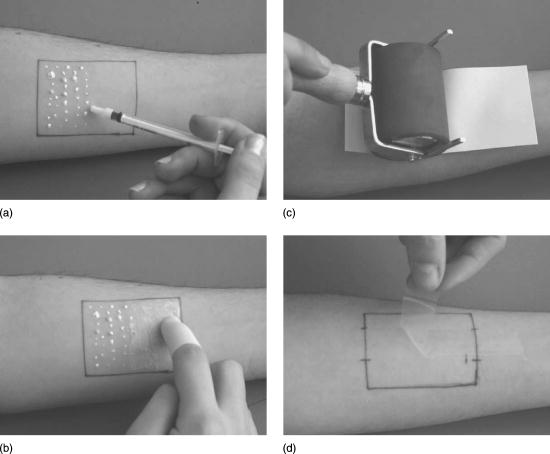
Removal techniques Removal techniques where substances deposited on the skin are removed generally by rinsing, wiping, or tape stripping. Figure 2 provides an overview of the tape stripping procedure. In this case, a substance is first applied to the skin (a & b) which do not always apply since investigators are often looking for environmental exposures, which does not require applying the agent. The last two images are the key steps in which a strip of adhesive tape is applied to an area of skin following exposure (c) then the tape is removed with the agent of interest (d) as well as several micrometers of the stratum corneum.
|
Figure 2 |
|
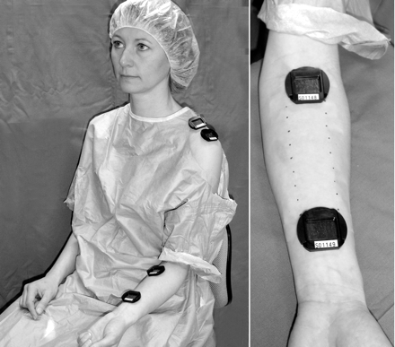
Surrogate skin techniques Surrogate skin techniques rely on a collection medium placed against the subject's skin, such as patches or gloves. Figure 3 provides an example of using patches both on the shoulder and forearm, which are used as collection media.
|
Figure 3 |
The article below by Stapleton et al looks to characterize exposure dermal exposure to PBDEs in household dust. More specifically, investigators wanted to examine the relationship between household dust, dermal exposure, and serum levels of PBDEs. Review the introduction and study methods prior to answering the questions below the article.
|
Image Citations
|
Ingestion is a common route of exposure for many different agents with the food we eat being a major source of exposure to many agents. Dietary exposure assessments help estimate exposure to both accidental and intentional substances and how that may affect one's health. This can include assessing the overall quantity and nutrition of food, the chemicals present in certain types of food, whether they are intentional chemicals such as those common in processed foods, or accidental chemicals as is the case in adulterated food (e.g. fruit containing pesticides or antibiotics).
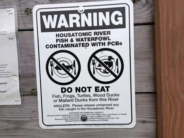
Shown below is a sign on the Housatonic River warning people not to eat animals from the river due to PCB contamination. General Electric will cover costs of an EPA-led cleanup of the river since the company had a factory on the river in Pittsfield, MA that released PCBs, which have recently been upgraded in the IARC Monographs to Group 1, known carcinogens.
Since dietary exposure assessments can focus on many different agents and a variety of exposure scenarios, this module will focus on dietary exposure to pesticides and some of the methods employed to estimate exposure to dietary pesticide intake.
The Environmental Working Group (EWG) is a non-profit organization that conducts research to assess the potential health impact from exposure to toxic chemicals via a myriad of sources with food being one. They release a report annually providing consumers a guide to pesticides in a variety of food sources. As part of their consumer guide, the EWG has identified the "dirty dozen" and the "clean fifteen" to identify which food products are among the most and the least contaminated with pesticides. Review the EWG Dirty Dozen list prior to answering the following question.
The Food Quality Protection Act (FQPA) was passed by Congress in 1996 and completely revised the nation's pesticide regulation since the 1960s. It mandates a health-based standard for pesticides used in foods, provides special protections to vulnerable populations (pregnant women, infants and children), and created a more streamlined process for approving of and incentivizing the use of safe pesticides.
A general algorithm for estimating dietary ingestion exposure of pesticides as well as the risk was established. The algorithm takes into account the frequency of pesticide residue detection and the levels, the number of pesticides detected in the single commodity, and the toxicity of the pesticides as shown in the formulas below.
|
Estimating Dietary Exposure and Risk to Pesticides |
|
1. Estimating dietary exposure to pesticides: To estimate dietary exposure, there are two components to consider in the formula: (1) average pesticide residue found on a given food product and (2) how much of a given food product is consumed on average. Both are discussed in greater detail in the next section. Exposureingestion = Residue x Consumption 2. Estimating risk from dietary exposure to pesticides: Once exposure has been estimated, risk can be determined by multiplying the exposure level by the hazard. Riskdietary = Hazard x Exposureingestion |
In order to determine dietary exposure to pesticides, one needs to determine how much pesticide residue is on a given food product and how much of that food product is consumed on average. These are two dependent variables where consumption determines exposure and residue magnifies/modifies the risk. Quantifying both residue and consumption are equally important and critical to estimating dietary exposure. The following table highlights both dietary consumption and pesticide residue databases.
|
Dietary Consumption Databases
Pesticide Residue Databases
|
Dietary consumption surveys such as NHANES can be a powerful tool for researchers since it is such a large database and includes many tutorials on how the database can be used. However, such cross-sectional surveys are limited in that they do not account for seasonal differences in food consumption. Thinking back to the "dirty dozen," this can be problematic since many of the seasonal foods/commodities can have incur higher risk for pesticide exposure. Furthermore, cross-sectional survey data is unable to reveal some of the unique consumption patterns within a region or subset of a population.
Longitudinal dietary data can be collected via person-to-person interviews similar to cross-sectional surveys. However, the use of person-to-person interviews can be very expensive and require the use of more time and resources. The table below highlights additional methods that can be employed to collected dietary day.
|
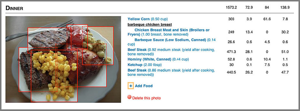
Digital Photos With the use of digital photography, images of the food selection and then the leftovers are captured are taken and analyzed using computer software to quantify how much food was consumed. This method started with researchers capturing food intake data in cafeterias and relied on trained individuals to capture the images as well as compare them to standard portions. The Remote Food Photography Methods was derived from this method to further expand on data collection beyond cafeterias and enable participants to take pictures of their food selections using smartphones and send to researchers via wireless data transfer.
|
|
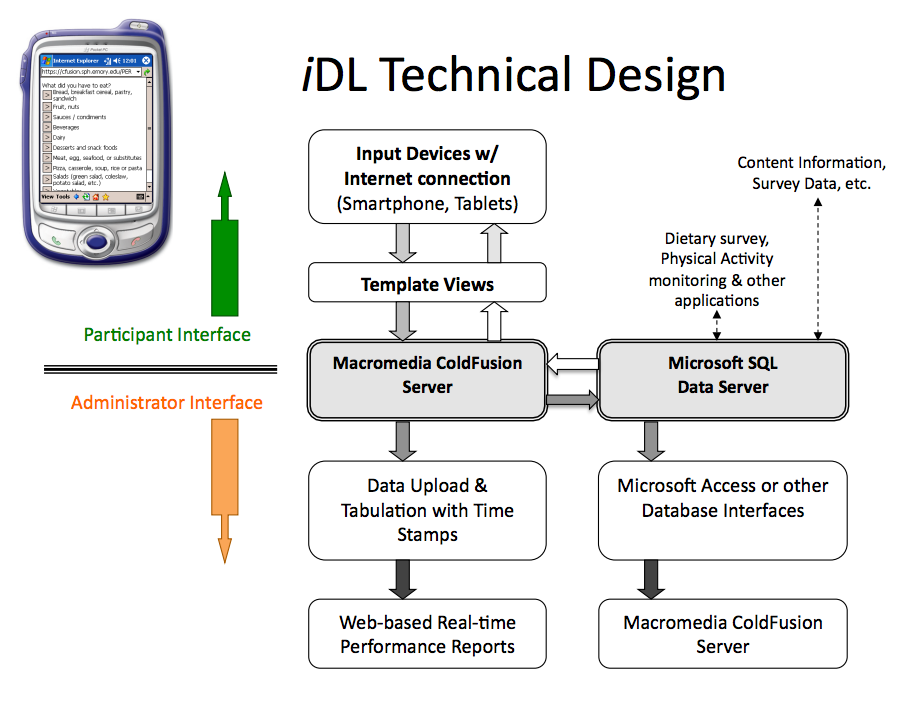
Internet Data Logger (iDL) The iDL is a real-time web-based system designed for optimal performance with mobile devices. It is comparable to an in-person interview without the inconvenience and constraints of in-person interviews. The survey data is received and compiled instantaneously. iDLs have the benefit of improving participant adherence to protocols and can be adaptive to other surveys if researchers wish to collect additional data, such as behavior, activity, medical records, etc.
|
Food that is contaminated by pesticide exposure is often contaminated with more than one type of pesticide. When determining dietary exposure to multiple pesticide residues, it is not correct to simply arithmetically add residues of different pesticides that have different toxicities. The relative potency factor (RPF) is a normalizing factor for the potency or toxicity among different pesticides in relation to the index pesticide. The amount of residue of each pesticide should be adjusted by multiplying by an RPF in order to obtain the equivalent residue of the index pesticide.
The table below shows the algorithm for estimating exposure to multiple residues (Exposureindex).
|
RPF-Based Multi-residue Algorithm |
|
Step 1. First calculate the index residue of each pesticide of interest by multiplying its residue by its residue potency factor. Residueindex (per OPx) = Residue x RPFx Step 2. Then calculate the index exposure for each pesticide of interest by multiplying the product of Step 1 with the average consumption of the food product of interest. Exposureindex = Residueindex x Consumption Step 3. To estimate cumulative exposure to all of the pesticides, find the sum of all the index exposures calculated in Step 2. Cumulative exposureindex = Σ (Residueindex x Consumption) |
The article below by Lu et al investigates children's dietary exposure to pesticides using a more direct measurement known as the 24-hr duplicate food samples in order to compare pesticide residues from direct measurements to those reported by the USDA Pesticide Data Program. Review the introduction and study methods prior to answering the questions below the article.
Exposure assessments looking to estimate exposure levels to noise have commonly been conducted in occupational health settings since certain occupations are potentially exposed to damaging levels of noise, such as construction workers and public safety workers. Traditionally the health outcome of concern was hearing loss which tends to be associated with occupational exposure levels. However, investigators are increasingly interested in examining the non-hearing-loss-related effects of environmental noise exposure.
There are two major types of sensori-neural hearing loss: age-related and noise-induced. Age-related hearing loss tends to be a cumulative effect of aging that results in loss in loudness where individuals tend to lose higher frequencies and it tends to affect men more than women. Noise-induced hearing loss results from damage to the hair cells or auditory nerves and includes loss of hearing clarity of low frequencies (vowels) and high frequencies (consonants). In addition to the effects on hearing, noise exposure can also result in non-auditory effects, such as annoyance, stress, hormone irregularity, cardiovascular disease, and interaction with other occupational and environmental exposures.

In order to assess the effects of noise on a given population, investigators must be able to measure and interpret noise data. The table below highlights some important definitions and measurements used to characterize noise exposure.
|
Key Definitions, Concepts and Formulas |
|
|
Sound: Vibration of spring-like air "particles" due to an oscillating surface, such as a vibrating tuning fork. |
|
|
Sound propagation: Vibrating particles exert a force on adjacent particles, causing them to vibrate thereby generating alternating regions of pressure that are slightly higher and lower than atmospheric pressure |
|
|
Sound waves: Consists of wavelengths, which are the distance between maxima (shown below) and frequency, which are the number of waves per second. The image below illustrates a speaker membrane sending trains of compression waves to the ear. Individual molecules oscillate about fixed positions.
|
|
|
Frequency: The number of cycles per unit of time often measured in Hertz (Hz). Frequency is related to the wavelength of sound. The wavelength is the distance in space required to complete a full cycle of a frequency. |
|
|
Sound pressure level (SPL): A logarithmic measure of the ratio between the actual sound pressure and a fixed reference pressure (formula below). The reference pressure used in the formula is usually that of the threshold of hearing, which is 20 μPa. SPL is typically used to measure magnitude of sound. Lp = 20 log10 p/p0
|
A 1dB change in sound level is not perceptible to the human ear. Generally it takes a change in noise by 5 dB before the change can be clearly perceived by the human ear and a change by 10dB is perceived as twice (or half) as loud. This is an important consideration when conducting exposure assessments. If an investigator is conducting an exposure assessment to characterize exposure to noise in different locations, even though there may be differences in noise levels from one location to another, these changes may not be meaningful unless they are large enough.
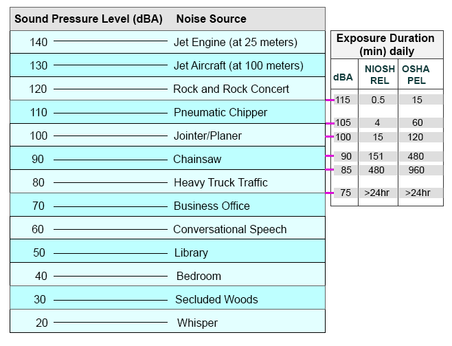
The diagram below provides examples of sources at different sound pressure levels with the table on the left. The appended table on the right includes the SPL and exposure duration under both NIOSH recommended exposure limits (RELs) and OSHA permissible exposure limits (PELs). Note the difference in exposure duration between what is recommended and what is permitted.
In order to collect data on noise, investigators must identify the sampling equipment that will best suit the objectives of the study. The table below provides some examples of the type of equipment that can be used to capture and collect noise data.
|
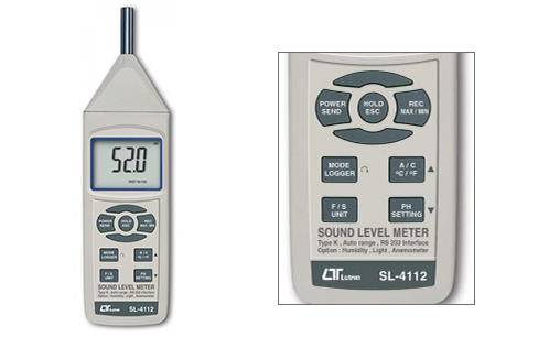
Sound Level Meter The sound level meter, shown in Figure 1, is an instrument that measures sound pressure level. It can be used to identify and evaluate individual noise sources for abatement purposes and can aid in determining the feasibility of engineering controls for individual noise sources. Another use of the sound level meter is to spot-check noise dosimeter performance.
|
Figure 1 |
|
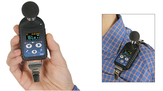
Noise Dosimeter A noise dosimeter is very similar to a sound level meter except that it can be worn by an employee to determine the personal noise dose during the workshift sampling period. Figure 2 illustrates how a noise dosimeter can be attached to clothing to capture personal exposure levels. They are often used to make compliance measurements according to OSHA noise standards. They can measure an employee's exposure to noise and automatically compute the necessary noise dose calculations.
|
Figure 2 |
|
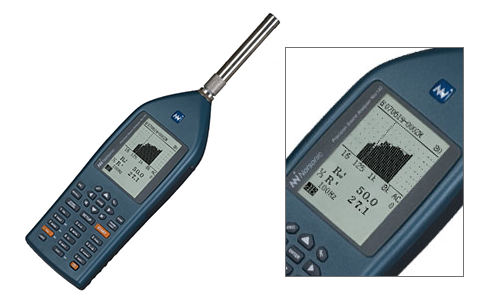
Octave Band Analyzer An octave band analyzer, shown in Figure 3, is a sound level meter that divides noise into its frequency components, which allows for further characterization of noise beyond a simple measure in decibels. Shown below is an example of octave band analysis. Note that the analysis allows for more detailed information regarding the breakdown of frequencies that make up the noise. It helps determine the effectiveness of various types of frequency-dependent noise controls, such as barriers and personal protective equipment (PPE). The special signature of any given noise can be obtained by taking sound level meter readings at each of the center frequency bands.
|
Figure 3 |
We have discussed measurements that are based on objective measures, specifically the decibel scale and the intensity levels it is based on. However, sounds with equal intensities but different frequencies are perceived to have unequal loudness. For example, an 80 dB sound with a frequency of 1000 Hz sounds louder than an 80 dB sound with a frequency of 500 Hz. To account for this subjective measure, the unit "phon" is used to indicate perception of loudness. One phon is equivalent to 1 dB at 1000 Hz. The diagram below displays equal loudness contours.
To compensate for this difference in loudness due to frequency, a frequency-dependent correction is made. The A-weighting scale is the most commonly used weighting scale for this correction. When sound pressure levels are corrected in this way, the units are designated as dBA, rather than dB.
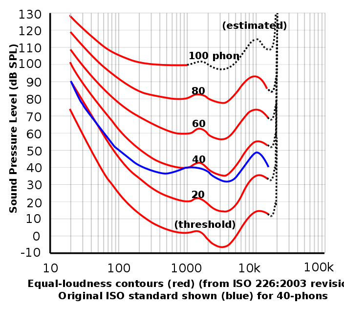
Figure 4
The article below by Dratva et al examines the effects of transportation noise on blood pressure with a secondary aim to look at these potential effects in vulnerable subpopulations. Review the introduction and study methods prior to answer the questions below the article.
|
Image Citations
|
Biological monitoring involves using biomarkers to represent or estimate exposure. A biomarker is a biochemical, molecular, genetic, immunologic, or physiologic indicator of events in a biological system. As a result, biomarkers are indicators of exposure, effect, and/or susceptibility. The diagram below shows an abbreviated version of the conceptual model for exposure-related disease. This diagram highlights variables that affect the pathway of internal exposure. What is important to note is how absorption, pharmacokinetics, and toxicodynamics affect the exposure-disease pathway and subsequently will determine which biomarkers can be used to estimate exposure.
Absorption: External dose of an agent is not necessarily equivalent to the internal dose, which is affected by how the agent is absorbed into the bloodstream. Factors such as the physical and chemical properties of a given agent, the route(s) of exposure, the presence of other chemicals will affect how much of the agent is actually absorbed by the body. DEHP is not as readily absorbed through the skin when compared to ingestion.
Pharmacokinetics: The pharmacokinetics of a given agent or chemical refer to once it is absorbed, how it it distributed, metabolized/biotransformed, and eliminated. These factors will elucidate where biomarkers can be found for a given agent. Some agents are more readily excreted in urine where others are excreted in feces, which may determine which collection medium will be used to measure biomarkers. For example, dioxins tend to be lipophilic and stored in adipose tissue whereas most of absorbed lead tends to be stored in bone tissue.
Toxicodynamics: Toxicodynamics describe the mechanism of action, meaning the interactions of a toxicant with a site of action (biological target) that result in a given effect. Using the diagram below for reference, this would be the altered structure or function preceding an adverse health outcome. For example, obesogens are xenobiotic compounds that interfere with normal development and balance of lipid metabolism, which can lead to obesity. Carcinogens tend to have different toxicodynamics that result in damage to normal cells by altering DNA or the regulation/expression of DNA.

The Exposure Biology Research Group (EBRG), directed by Dr. Michael McClean, is an interdisciplinary research group in the department of Environmental Health at the Boston University School of Public Health. Their research focuses on the use of biological markers to assess environmental and occupational exposures.
"Biomarkers: Potential Uses and Limitations" is an article by Richard Mayeux that discusses some of the benefits and limitations to using biomarkers with respects to studying neurological diseases. Below is a summary of some of the general advantages and disadvantages of using biomarkers as indicators of exposure.
Advantages to using biomarkers: Biological monitoring allows investigators to integrate exposure via multiple pathways and can be easier to measure for long-term exposure. As a direct measure of exposure, biomarkers are free from recall bias and tend to reveal useful information on the ADME of the exposure. Biomarkers are also found close to the health outcome along the exposure-related disease pathway, so they are often relevant to the outcome of interest. Inter-individual variability with biomarkers provides important information in terms of how exposure can impact individuals differently while intra-individual variability provides some insight on how exposure changes over time. Biomarkers are also an excellent tool for evaluating the effectiveness of implemented exposure controls as well as personal protective equipment.
Disadvantages to using biomarkers: The use of biological monitoring can be expensive and require some intrusive techniques to collect data from participants. Furthermore, most biomarkers are experimental and there is limited data on "normal" populations. Other concerns are the variability in analytical techniques that can take place either within a lab or among different labs can yield different results. While inter- and intra-variability of biomarkers can provide some useful information regarding exposure, it can also pose some limitations when trying to extrapolate data collected on a sample population to the general population.
The validity of a biomarkers depends on the following variables: sensitivity, specificity, reproducibility, stability, temporal relevance, practicality. Scroll through the tabbed activity below to learn more about these important considerations when using biomarkers.
Because biomarkers consists of such a wide range of biological indicators, there are many ways to measure biomarkers as well as many different types of biomarkers. The best method will depend on the exposure of interest as well as feasibility in terms of the resources available, such as equipment and staff. Another important consideration is how invasive the procedure is in terms of collecting biomarker data from the study population. This usually involves the collection of the biomarker in a matrix (e.g. hair, skin, saliva, etc.). The following table includes examples of both invasive and non-invasive matrices through which biomarker data can be collected.
|
Non-invasive Matrices In addition to being minimally invasive making subjects more likely to participate, Most of the matrices listed below require little to no advanced skills for collection.
|
|
Invasive Matrices Invasive procedures to collect biomarker data can be off-putting to potential study participants. Most of the matrices listed below require advanced skills for proper collection, which can also affect resources and time available.
|
The article below by Rudel et al identifies biomonitoring measurement methods for chemicals that cause mammary gland tumors in animals in order to identify potential biomonitoring tools for breasts cancer studies and surveillance in humans. Review the introduction and study methods prior to answering the questions below the article.