


Tests with Matched Samples, Continuous Outcome
In the previous section we compared two groups with respect to their mean scores on a continuous outcome. An alternative study design is to compare matched or paired samples. The two comparison groups are said to be dependent, and the data can arise from a single sample of participants where each participant is measured twice (possibly before and after an intervention) or from two samples that are matched on specific characteristics (e.g., siblings). When the samples are dependent, we focus on difference scores in each participant or between members of a pair and the test of hypothesis is based on the mean difference, μd. The null hypothesis again reflects "no difference" and is stated as H0: μd =0 . Note that there are some instances where it is of interest to test whether there is a difference of a particular magnitude (e.g., μd =5) but in most instances the null hypothesis reflects no difference (i.e., μd=0).
The appropriate formula for the test of hypothesis depends on the sample size. The formulas are shown below and are identical to those we presented for estimating the mean of a single sample presented (e.g., when comparing against an external or historical control), except here we focus on difference scores.
Test Statistics for Testing H0: μd =0
- if n > 30


- if n < 30
 where df =n-1
Example:
A new drug is proposed to lower total cholesterol and a study is designed to evaluate the efficacy of the drug in lowering cholesterol. Fifteen patients agree to participate in the study and each is asked to take the new drug for 6 weeks. However, before starting the treatment, each patient's total cholesterol level is measured. The initial measurement is a pre-treatment or baseline value. After taking the drug for 6 weeks, each patient's total cholesterol level is measured again and the data are shown below. The rightmost column contains difference scores for each patient, computed by subtracting the 6 week cholesterol level from the baseline level. The differences represent the reduction in total cholesterol over 4 weeks. (The differences could have been computed by subtracting the baseline total cholesterol level from the level measured at 6 weeks. The way in which the differences are computed does not affect the outcome of the analysis only the interpretation.)
|
Subject Identification Number |
Baseline |
6 Weeks |
Difference |
|---|---|---|---|
|
1 |
215 |
205 |
10 |
|
2 |
190 |
156 |
34 |
|
3 |
230 |
190 |
40 |
|
4 |
220 |
180 |
40 |
|
5 |
214 |
201 |
13 |
|
6 |
240 |
227 |
13 |
|
7 |
210 |
197 |
13 |
|
8 |
193 |
173 |
20 |
|
9 |
210 |
204 |
6 |
|
10 |
230 |
217 |
13 |
|
11 |
180 |
142 |
38 |
|
12 |
260 |
262 |
-2 |
|
13 |
210 |
207 |
3 |
|
14 |
190 |
184 |
6 |
|
15 |
200 |
193 |
7 |
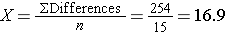
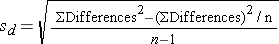
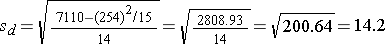
Because the differences are computed by subtracting the cholesterols measured at 6 weeks from the baseline values, positive differences indicate reductions and negative differences indicate increases (e.g., participant 12 increases by 2 units over 6 weeks). The goal here is to test whether there is a statistically significant reduction in cholesterol. Because of the way in which we computed the differences, we want to look for an increase in the mean difference (i.e., a positive reduction). In order to conduct the test, we need to summarize the differences. In this sample, we have
- N=15

- sd=14.2
The calculations are shown below.
|
Subject Identification Number |
Difference |
Difference2 |
|---|---|---|
|
1 |
10 |
100 |
|
2 |
34 |
1156 |
|
3 |
40 |
1600 |
|
4 |
40 |
1600 |
|
5 |
13 |
169 |
|
6 |
13 |
169 |
|
7 |
13 |
169 |
|
8 |
20 |
400 |
|
9 |
6 |
36 |
|
10 |
13 |
169 |
|
11 |
38 |
1444 |
|
12 |
-2 |
4 |
|
13 |
3 |
9 |
|
14 |
6 |
36 |
|
15 |
7 |
49 |
| Totals |
254 |
7110 |
Is there statistical evidence of a reduction in mean total cholesterol in patients after using the new medication for 6 weeks? We will run the test using the five-step approach.
- Step 1. Set up hypotheses and determine level of significance
H0: μd = 0 H1: μd > 0 α=0.05
NOTE: If we had computed differences by subtracting the baseline level from the level measured at 6 weeks then negative differences would have reflected reductions and the research hypothesis would have been H1: μd < 0.
- Step 2. Select the appropriate test statistic.
Because the sample size is small (n<30) the appropriate test statistic is
.
- Step 3. Set up decision rule.
This is an upper-tailed test, using a t statistic and a 5% level of significance. The appropriate critical value can be found in the t Table at the right, with df=15-1=14. The critical value for an upper-tailed test with df=14 and α=0.05 is 2.145 and the decision rule is Reject H0 if t > 2.145.
- Step 4. Compute the test statistic.
We now substitute the sample data into the formula for the test statistic identified in Step 2.
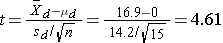
- Step 5. Conclusion.
We reject H0 because 4.61 > 2.145. We have statistically significant evidence at α=0.05 to show that there is a reduction in cholesterol levels over 6 weeks.
Here we illustrate the use of a matched design to test the efficacy of a new drug to lower total cholesterol. We also considered a parallel design (randomized clinical trial) and a study using a historical comparator. It is extremely important to design studies that are best suited to detect a meaningful difference when one exists. There are often several alternatives and investigators work with biostatisticians to determine the best design for each application. It is worth noting that the matched design used here can be problematic in that observed differences may only reflect a "placebo" effect. All participants took the assigned medication, but is the observed reduction attributable to the medication or a result of these participation in a study.
Video - Hypothesis Testing With a Matched Sample and a Continuous Outcome (3:11)
Link to transcript of the video
![]()
![]()