PH717 Module 1B - Descriptive Tools
Descriptive Epidemiology & Descriptive Statistics
Disease surveillance systems and health data sources provide the raw information necessary to monitor trends in health and disease. Descriptive epidemiology provides a way of organizing and analyzing these data in order to understand variations in disease frequency geographically and over time, and how disease (or health) varies among people based on a host of personal characteristics (person, place, and time). This makes it possible to identify trends in health and disease and also provides a means of planning resources for populations. In addition, descriptive epidemiology is important for generating hypotheses (possible explanations) about the determinants of health and disease. By generating hypotheses, descriptive epidemiology also provides the starting point for analytic epidemiology, which formally tests associations between potential determinants and health or disease outcomes. Specific tasks of descriptive epidemiology are the following:
In this module we will provide you with the key elements of descriptive epidemiology and the descriptive statistics that are fundamental to defining the health status of populations, identifying health problems, and generating hypotheses about the determinants of health and disease.
After completing this this week's learning activities, you will be able to:
Part 1 - Descriptive Epidemiology
Keeping track of the frequency of health problems in a population is essential to the planning, implementation, and evaluation of public health practice, and this information needs to be readily available to those responsible for prevention and control of disease. How is the raw data for this endeavor obtained and evaluated?
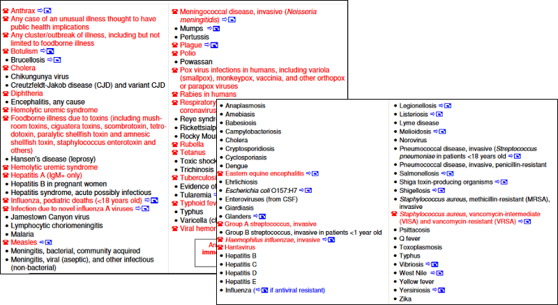
Today there are many sources of data that are useful for monitoring the health of populations and for exploring how disease frequency changes over time and how it relates to personal characteristics and location (person, place and time). Below is a partial list of examples of possible data sources.
There are many cross-sectional surveys and databases that are periodically conducted, many of which can be accessed from the National Center for Health Statistics.
Descriptive epidemiology searches for patterns by examining characteristics of person, place, & time . These characteristics are carefully considered when a disease outbreak occurs, because they provide important clues regarding the source of the outbreak.
Hypotheses about the determinants of disease arise from considering the characteristics of person, place, and time and looking for differences, similarities, and correlations. Consider the following examples:
Descriptive epidemiology provides a way of organizing and analyzing data on health and disease in order to understand variations in disease frequency geographically and over time and how disease varies among people based on a host of personal characteristics (person, place, and time). Epidemiology had its origins in the desire to understand the determinants of acute infectious diseases, but its methods and applicability have expanded to include chronic diseases as well.
There are many personal characteristics and behaviors that are relevant to health status and might be considered "exposures" or risk factors that ought to be considered when conducting research on the determinants of disease or when trying to predict risk. Age, sex, and race/ethnicity are almost always variables of potential interest since the frequency of health outcomes can vary markedly with these characteristics. However, one should think broadly about the many other personal characteristics that might be important, such as:
Where one lives, works, and travels can provide clues about relevant exposures. In addition, surveillance data showing how disease frequency varies geographically, or even within the same workplace, might provide valuable clues about the etiology of a health problem.
Example 1: Stomach Cancer by Location in the US
The maps below show death rates from stomach cancer in females and males in different US counties. The darkness of shading of each county indicates how its stomach cancer rate compares with the national average. The darkest shading indicates rates well above average, and white shading indicates rates below average; the gray shading indicates intermediate levels. Note that rates of stomach cancer tend to be high in counties in the north-central part of the country in both males and females. Investigators speculated that these clusters might correlate with populations of German or Scandinavian descent who have a tradition of eating smoked fish. Could the high rates of stomach cancer be the result of their consumption of smoked fish or other traditional methods of food preservation?
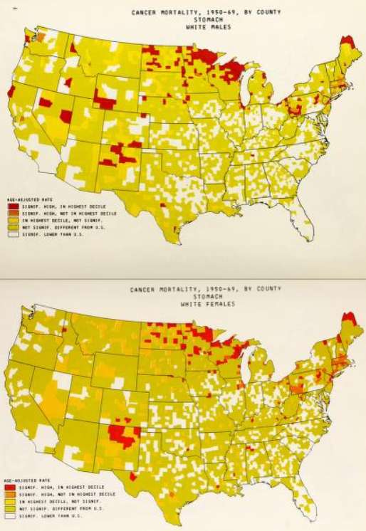
Source: Atlas of Cancer Mortality for U.S. Counties: 1950-1969, TJ Mason et al, PHS, NIH, 1975
https://archive.org/details/atlasofcancermor00nati_0
Example 2: Differences in Rates of Stomach Cancer in Japan and US
Rates of stomach cancer also vary among countries. Japanese have a higher rate of stomach cancer than Caucasians in California. Is this due to a genetic difference? A dietary difference? The rate among Japanese people diminishes after they move to US, and diminishes even more in their offspring. One possibility is that once the Japanese move here, they begin to shift to an American diet, and this trend is even stronger in their children. Are there important dietary differences? Could consumption of large amounts of smoked fish be a cause of stomach cancer?
| Population |
Mortality Rate (per 100,000 population) |
|
Japanese in Japan |
58.4 |
|
Japanese immigrants to California |
29.9 |
|
Sons of Japanese immigrants |
11.7 |
|
Native Californians (Caucasians) |
8.0 |
Public health surveillance systems provide the data to monitor the frequency of health problems over time, and this is vitally important for identifying outbreaks and trends in disease frequency over time. One should consider changes in disease frequency on several different scales depending upon the disease of interest.
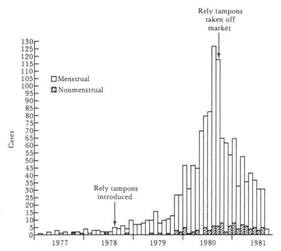
Example: Toxic Shock and Rely Tampons
In January 1980 there were several reports of toxic shock syndrome due to infection with Staphylococcus aureus bacteria, and the descriptive epidemiology indicated that the problem was occurring primarily in menstruating women. A CDC task force investigated and eventually traced the outbreak to the introduction of Rely tampons, a super absorbent product marketed by Proctor and Gamble. The monthly cases of toxic shock syndrome in 1980-1981 are shown in the graph below [from A. Reingold et al., Toxic shock syndrome surveillance in the United States, 1980-1981. Ann. Intern. Med 96:875, 1982]. The graph shows that prior to 1978 there were just occasional cases of toxic shock syndrome in the United States. After Rely tampons were introduced in 1978, there was a steady increase in toxic shock cases which peaked at about 125 per month in 1980. Shortly after that, Rely tampons were taken off the market, and the incidence declined sharply.
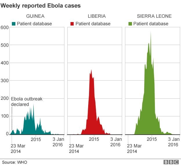
There were also dramatic changes in the frequency of the Ebola epidemic in Africa in 2017, as shown below. The epidemic curves for Guinea, Liberia, and Sierra Leone show that the number of Ebola cases began to rise in March 2014, peaked in mid 2015, and then gradually fell by January 2016.
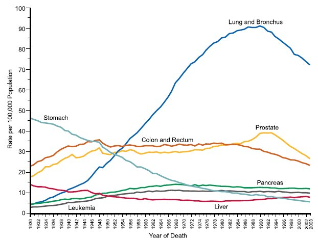
The incidence of some cancers has varied over time as a result of changes in behavior or diagnostic methods and treatment. Decreases in tobacco smoking were followed by a decline in frequency of lung cancer, and modern methods of food preservation led to a decrease in stomach cancer. The diagnosis of prostate cancer increased after introduction of the PSA (prostate specific antigen) test, and mortality from colorectal decreased after the introduction of colonoscopy as a screening and treatment modality. These changes are demonstrated in the graph below, which shows changes in the incidence of selected cancers over time in males.
Categories of Descriptive Epidemiology
A case report is a detailed description of disease occurrence in a single person. Unusual features of the case may suggest a new hypothesis about the causes or mechanisms of disease.
Example: Acquired Immunodeficiency in an Infant; Possible Transmission by Means of Blood Products
In April 1983 it had not yet been shown that AIDS could be transmitted by blood or blood products. An infant born with Rh incompatibility; required blood products from 18 donors over 8 weeks and subsequently developed unusual recurrent infections with opportunistic agents such as Candida. The infant's T cell count was low, suggesting AIDS. There was no family history of immunodeficiency, but one of the blood donors was found to have died of AIDS. This led the investigators to hypothesize that AIDS could be transmitted by blood transfusion.
Link to article by Ammann AJ et al: Acquired immunodeficiency in an infant: possible transmission by means of blood products. The Lancet 1:956-958, 1983.
A case series is a report on the characteristics of a group of subjects who all have a particular disease or condition. Common features among the group may suggest hypotheses about disease causation. Note that the "series" may be small (as in the example below) or it may be large (hundreds or thousands of "cases"). However, the chief limitation is that there is no comparison group. Consequently, common features may suggest hypotheses, but these need to be tested with some sort of analytical study before an association can be accepted as valid.
Example: Discovery of HIV in the United States
 In 1980 -1981 four previously healthy young men were diagnosed with Pneumocystis carinii pneumonia, an unusual "opportunistic" infection that had only been seen in immune compromised people with hereditary disorders or in people with immune compromise due to chemotherapy. The medical histories didn't suggest any preexisting immunodeficiency, but all four men had decreased immune responses and low T cell counts. These unusual infections suggested the possibility of a previously unknown disease. It was noted that all four men were sexually active homosexuals, and in the case series which was published in the New England Journal of Medicine the authors speculated that the immune dysfunction was due to a sexually transmitted infectious agent.
This was an extraordinarily important case series (a detailed description of characteristics of a series of people who all have the same disease) that suggested that this new syndrome was associated with sexual activity in male homosexuals. Alerting the medical establishment and proposing a hypothesis was an important milestone in the AIDS epidemic.
Link to article by Gottlieb MS, et al: Pneumocystis carinii pneumonia and mucosal candidiasis in previously healthy homosexual men: evidence of a new acquired cellular immunodeficiency. N Engl J Med 1981;305:1425-1431.
 Oral Contraceptives and Hepatocellular Carcinoma?
There had been a number of case reports of liver cancers in young women taking oral contraceptives. A study was undertaken by contacting all of the cancer registries collaborating with the American College of Surgeons. The investigators wanted to collect information on as many of these rare liver tumors as possible across the US.
Table - Oral Contraceptive Use Among Women Who Developed Liver Cancer
| Oral Contraceptive Use |
Age 16-25 yrs. |
Age 26-35 yrs. |
Age 36-45 yrs. |
|
Yes |
31% |
43% |
22% |
|
No |
20% |
10% |
29% |
|
Unknown |
49% |
48% |
49% |
What conclusions can you draw from these data regarding a possible increased risk of liver cancer in woman taking oral contraceptives? Think about it before you look at the answer.
Answer
|
Key Concept: The key to identifying a case series is that all of the subjects included in the study have the primary disease or outcome of interest. For example, an article reported on 239 people who got bird flu. The article might present tables and graphs that gave information about their age, occupation, where they lived, whether they lived or died, etc., but basically it is a detailed description of the characteristics and outcomes in a group of people who all had the same disease.
|
|
Strengths of Case Reports and Case Series
|
|
Limitations of Case Reports and Case Series
|
Cross-sectional surveys assess the prevalence of disease and the prevalence of risk factors at the same point in time and provide a "snapshot" of diseases and risk factors simultaneously in a defined population. For example, US government agencies periodically send out large surveys to random samples of the US population, asking about health status and risk factors and behaviors at that point in time. The Health Interview Survey (HIS) and the National Health and Nutrition Examination Survey (NHANES) are good examples.
The health questionnaires you are asked to fill out when you go to a new physician or being processed for a new job, or prior to entry into military service are similar to cross-sectional surveys in that they ask about the health problems that you have (heart disease? diabetes? asthma?) and your current behaviors and risk factors (e.g., How old are you? Do you smoke? What is your occupation?).
Cross-sectional surveys ask people their current status with respect to both exposures and diseases. They are often referred to as "prevalence studies," because they assess the prevalence of exposures and health outcomes at a point in time. They have two main disadvantages.

|
Limitations of Cross-sectional Surveys:
These limitations are discussed below. |
Temporal Relationship Between Exposure and Outcome
Consider the following example in which a survey was conducted among white male farm workers. The survey asked many questions, but among them were the questions: "Have you been told you have coronary heart disease (CHD)?" And "How would you classify your level of physical activity?" The table below summarizes the findings.
Table - Current Activity and Coronary Heart Disease Among Male Farm Workers
|
# of Respondents |
# Respondents With CHD |
Prevalence of CHD per 1,000 |
|
|
Currently Not Active |
89 |
14 |
157 |
|
Currently Active |
90 |
3 |
38 |
Note that the investigators did not follow these subjects over a period of time, so they did not assess the "incidence" of heart disease. Instead, they asked the subjects questions designed to determine the prevalence of heart disease, i.e., the proportion of the study population that had heart disease at this particular point in time. When they divided the sample into physically active and inactive farmers and computed the prevalence of heart disease in each of these, they found that CHD was much more prevalent among the inactive farmers. However, this was a cross-sectional study that related the prevalence of disease to the prevalence of activity at a point in time. They did not follow subjects over time to track the development of heart disease (i.e., the incidence). Consequently, the temporal relationship between the risk factor of interest (physical inactivity) and the outcome (CHD) is unclear.
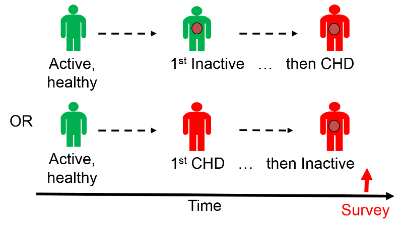
Had the farmers been physically active prior to developing CHD? Or, did they begin to limit their physical activity after they developed CHD? It is unclear. Consequently physical inactivity could have been either a cause of heart disease, or it could have been a consequence of CHD.
Large cross-sectional surveys are important for monitoring health status and health care needs of the population over time, and they are sometimes useful for suggesting possible associations between risk factors and diseases. However, the temporal relationship between the risk factor and disease is frequently unclear. Under these circumstances, they can generate hypotheses, but these associations need to be tested by appropriate analytical studies.
However, note that under some circumstances, the temporal relationship is clear on a cross-sectional survey. For example, if one conducted a survey of salaries of male and female professors to see if sex was associated with salary inequities, we could regard this as an analytical study, because it is clear that sex was established long before salary level. In this situation the temporal relationship between the "exposure" of interest (sex) and outcome (salary paid) is clear; we know that gender was established before the salary was negotiated. So, in a sense cross-sectional studies (and ecological studies can be thought of as an intermediate category between descriptive and analytic studies.
Identification of Cases of Long Duration
A second limitation of cross-sectional studies is that they are more likely to identify cases of long duration, and this can bias the results.
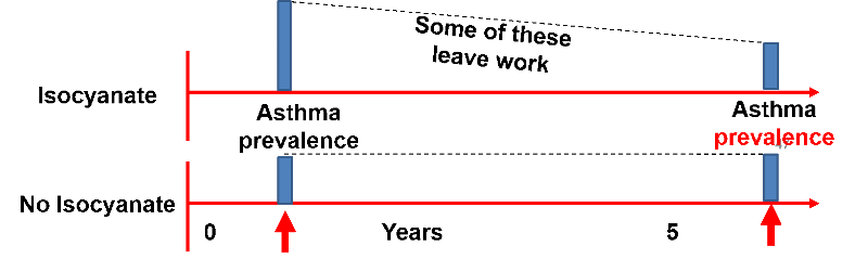
Example: Isocyanates are chemicals that can cause occupational asthma that gets progressively worse over time. In a cross-sectional study of isocyanates and occupational asthma, the prevalence of asthma was lower in factory workers with >5 years employment vs. those with <5 years employment, because those with isocyanate exposure and asthma were more likely to leave.
Below is a hypothetical time line showing the apparent prevalence of occupational respiratory problems in workers exposed to isocyanates and unexposed workers. After one year of working the prevalence of respiratory problems is two-fold greater in the isocyanate workers, but by seven years the prevalence is similar, because the isocyanate workers who developed respiratory problems left and found other work.

Ecologic studies assesses the overall frequency of disease in a series of populations and looks for a correlation with the average exposure in the populations. These studies are unique in that the analysis is not based on data on individuals. Instead, the data points are the average levels of exposure and the overall frequency of disease in a series of populations. Therefore, the unit of observation is not a person; rather, it is an entire population or group.
In the study below investigators used commerce data to compute the overall consumption of meat by various nations. They then calculated the average (per capita) meat consumption per person by dividing total national meat consumption by the number of people in a given country. There is a clear linear trend; countries with the lowest meat consumption have the lowest rates of colon cancer, and the colon cancer rate among these countries progressively increases as meat consumption increases.
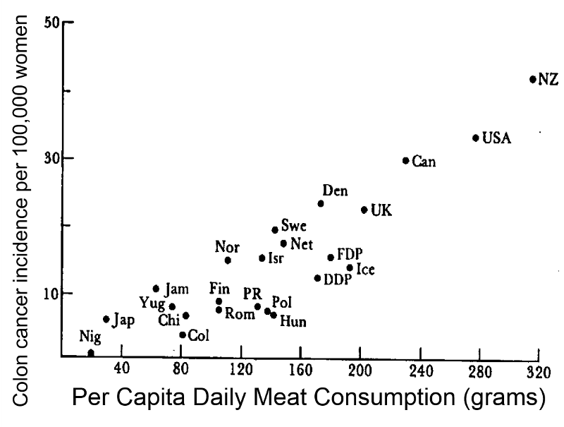
Note that in reality, people's meat consumption probably varied widely within each nation, and the exposure that was calculated was an average that assumes that everyone ate the average amount of meat. This average exposure was then correlated with the overall disease frequency in each country. The example here suggests that the frequency of colon cancer increases as meat consumption increases. The characteristic of ecological studies that is most striking is that there is no information about individual people. If the data were summarized in a spread sheet, you would not see data on individual people; you would see records with data on average exposure in multiple groups .
|
Advantages of Ecologic Studies
|
|
Limitations of Ecologic Studies
|
Example:
An ecological study correlated per capita alcohol consumption to death rates from coronary heart disease (CHD) in different countries, and it appeared that there was a fairly striking negative correlation as shown in the graph below.
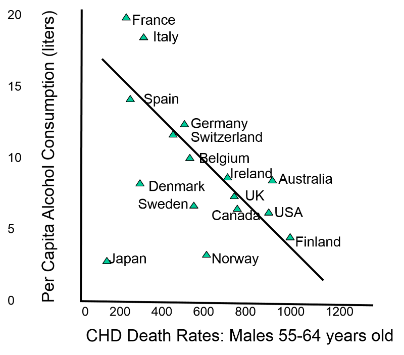
However, a cohort study with data on alcohol consumption in individual subjects showed that there was a J-shaped relationship. People who drank modestly had a lower mortality rates than those who did not drink at all, but among higher levels of individual consumption there was a striking linear increase in mortality, as shown in the graph below.
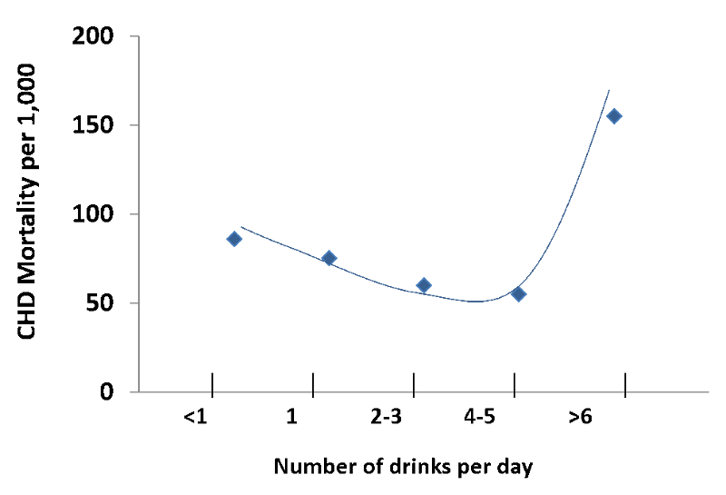
Source: Adapted from AR Dyer et al. Alcohol consumption and 17-year mortality in the Chicago Western Electric Company Study. Prev. Med. 1980; 9(1):78-90.
The real question was whether individuals who drank heavily had higher or lower mortality rates than those who drank modestly or not all, but the ecologic study led to an incorrect conclusion because it was based on aggregate data. In reality, most people drink modestly, but mortality rates are much greater in the small number of people who drink very heavily. The misleading conclusion from the ecologic study is an example of the ecologic fallacy.

To see an extraordinary example of an ecologic study, play the video below created by Hans Rosling. This is a magnificent example that examines the correlation between income and life expectancy in the countries of the world over time. It is also a terrific example of a creative, engaging, and powerful way to display a vast quantity of data.
Part 2 - Introduction to Descriptive Statistics
A descriptive measure for an entire population is a ''parameter.'' There are many population parameters. For example, the population size (N) is one parameter, and the mean diastolic blood pressure or the mean body weight of a population would be other parameters that relate to continuous variables. Other population parameters focus on discrete variables, such as the percentage of current smokers in the population or the percentage of people with type 2 diabetes mellitus. Health-related behaviors can also be thought of this way, such as the percentage of the population that gets vaccinated against the flu each year or the percentage who routinely wear a seatbelt when driving.
It is generally not feasible to directly measure parameters, since it requires collecting information from all members of the population. We therefore take samples from the population, and the descriptive measures for a sample are referred to as ''sample statistics'' or simply ''statistics.'' For example, the mean diastolic blood pressure, the mean body weight, and the percentage of smokers in a sample from the population would be sample statistics. In the image below the true mean diastolic blood pressure for the population of adults in Massachusetts is 78 millimeters of mercury (mm Hg); this is a population parameter. The image also shows the mean diastolic blood pressure in three separate samples. These means are sample statistics which we might use in order to estimate the parameter for the entire population. However, note that the sample statistics are all a little bit different, and none of them are exactly the sample as the population parameter.
Descriptive statistics are important for monitoring a population (surveillance), for analyzing and communicating trends in both acute and chronic disease frequency and trends in health-related behaviors (e.g., smoking, exercise, alcohol and drug use, seatbelt use, etc.) and many other relevant exposures. Descriptive statistics are also essential for analyzing and communicating the results of descriptive epidemiological studies (case series, cross-sectional studies, and ecologic studies. A variable is anything that has a quantity or quality that varies. We refer to health outcomes and dependent variables , because their occurrence depends on the presence of one or (usually) more than one exposures or risk factors, which are called independent variables. The variables (both exposures and health outcomes) that are collected for these purposes can be of several types.
Dichotomous, ordinal, and categorical variables are typically summarized by showing the sample size (N), the counts in each group, and the relative frequency or percentage in each group as illustrated by the variables for sex and race/ethnicity in the table below describing some of the baseline characteristics in a randomized clinical trial comparing outcomes in subjects treated with acetaminophen (Tylenol) or ibuprofen.
| Variable |
Acetaminophen N=150) |
Ibuprofen (N=150) |
|
Age in months |
40.3 +12.9 |
39.4 + 13.6 |
|
Male sex - no. (%) |
86 (57) |
93 (62) |
|
Race or ethnic group - no. (%) |
|
|
|
White |
74 (49) |
74 (49) |
|
Black |
47 (31) |
50 (33) |
|
Hispanic or Latino |
35 (33) |
37 (25) |
Continuous variables are generally summarized by indicating the number of subjects, an estimate of a central tendency value (a mean or a median ), and an indication of the degree of variability in the measurements ( standard deviation or interquartile range.) In the table below from the same study note that age is reported as mean + standard deviation, because it was a normally distributed continuous variable. IgE antibody levels and eosinophil counts in blood are reported as median and interquartile range because they were not normally distributed.
|
Variable |
Acetaminophen N=150) |
Ibuprofen (N=150) |
|
Age in months |
40.3 +12.9 |
39.4 + 13.6 |
|
Median IgE (interquartile range - kU/liter |
64 (19-176) |
70 (24-252) |
|
Median blood eosinophil count (interquartile range) - cells/mm3 |
259.6 (172.5-534.8 |
248.4 (132.8-450.0) |
There are two commonly used methods for describing the central tendency, or most central value of a continuous variable.
The mean is the average value, which is computed by summing the measurements and dividing by the number of observations. For example, suppose seven patients with cardiovascular disease have the following systolic blood pressures:
100 110 114 121 130 130 160
The sum is 865 and the mean is 865/7= 123.6.
The median is the middle value, i.e., the value at which half of the measurements are below that value and half are above. For the small sample of seven subjects above the media systolic blood pressure is 121 mm of mercury since half of the values are below this median and half are above. (To find the median one can sort the values and find the middle value if the number of values is odd; If the number of values is even, the median is the average of the two middle values. However, the R package can do this easily.)
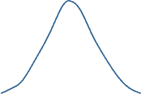
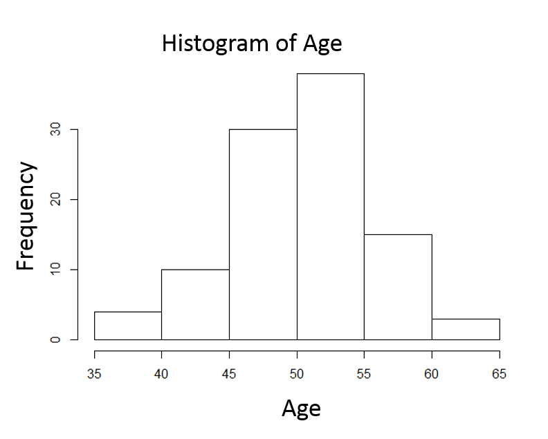
Consider the frequency distribution for the age of landscape workers in the image below.

The frequency distribution of age values is fairly symmetrical with the highest frequencies close to the middle and increasingly less frequent observations moving away from the center in either direction. One might describe the distribution as "bell-shaped," and this is an example of a normal distribution . One typically describes the central tendency with a mean. (Note that the mean and median will be similar in a symmetrical distribution like this.) The mean is calculated by adding all of the values and dividing the sum by the number of observations.
For a normal distribution the degree of variability or spread is indicated by the sample variance and the sample standard deviation .
Sample Variance and Sample Standard Deviation:
The sample variance is computed by first finding the mean and using it to compute the sum of the squares of the deviation of each value from the mean. The variance is the sum of the squared deviations divided by the sample size minus 1 (i.e., n-1).
 |
|
|
|
100 |
-23.6 |
556.96 |
|
110 |
-13.6 |
184.96 |
|
114 |
-9.6 |
92.16 |
|
121 |
-2.6 |
6.76 |
|
130 |
6.4 |
40.96 |
|
130 |
6.4 |
40.96 |
|
160 |
36.4 |
1324.96 |
|
865 |
0 |
2247.72 |
The sample standard deviation is simply the square root of the variance.
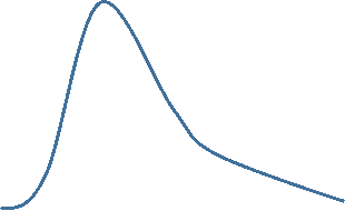
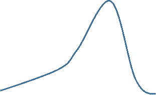
Now consider the frequency distribution of length of stay in the hospital in days as shown below.
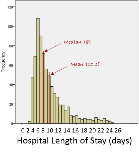
The distribution is not normal; it is skewed to the right . Frequency of length of stay rises to a peak at about 7 days and then very gradually falls with a few patients having stays as long as 24 to 25 days. For a distributed skewed to the right like this the median is a better characterization of the central tendency; the mean is pulled to the right by the extremely long length of stay in small numbers of patients. For skewed distributions like this or distributions with extreme outliers in either direction, one uses the median to characterize the central tendency, and the variability in the observations is described using the interquartile range described below.
Example of the effect of an extreme outlier:
100 110 114 121 130 130 360
This small data set is similar to the one that was previously used except that the last value has been replaced with an "outlier." The median is still 121, but the mean has now been pulled from 123.6 up to 152. So, for data sets with extreme outliers, one should use the median.
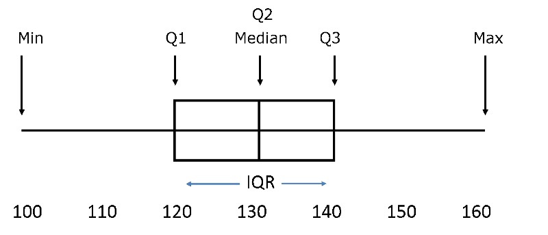
For clarity, the illustration below of a normal distribution will be used to explain quartiles and interquartile range. However, interquartile range is generally used for data that is not normally distributed.
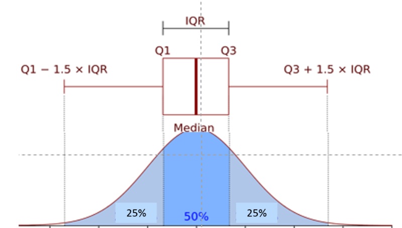
First, the observations are ranked from smallest to greatest, and the data set is divided into four equal parts ( quartiles ) such that each quartile has an equal (or nearly equal) number of observations. Half of the observations will be below the median, and half will be above. The 1st quartile (Q1) has the lowest 25% of observations, defined by finding the middle value between the lowest and median values. The 4th quartile (Q4) has the highest 25% of observations and is defined by finding the middle value between the median and the highest value in the data set. The 2nd quartile (Q2) has the 25% between the 1st quartile and the median, and the 3rd quartile (Q3) has the 25% between the median and the 4th quartile.
The interquartile range (IQR) is the range for the middle 50% of the data, i.e., between Q1 and Q3:

Example: Consider this small data set:
100, 110, 114, 121, 130, 130, 360
It would be very tedious to compute the IQR by hand, but statistical packages like R make it easy. Here is a preview:
> data<- c(100,110,114,121,130,130,360)
> summary(data)
Min. 1st Qu. Median Mean 3rd Qu. Max.
100.0 112.0 121.0 152.1 130.0 360.0
The lines in blue are commands to R. The first line of code above just creates this small data set, and the second line asks for a summary of the data.

Definitions of Outliers
Outliers are extreme values that meet either of these two conditions:
Summary:
For roughly symmetrical distributions use mean and standard deviation
For a right skewed distribution use median and IQR
For a left skewed distribution use median and IQR


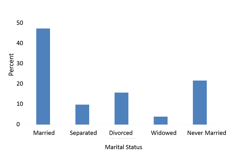
A bar chart indicates separate categories by spaces between the bars.
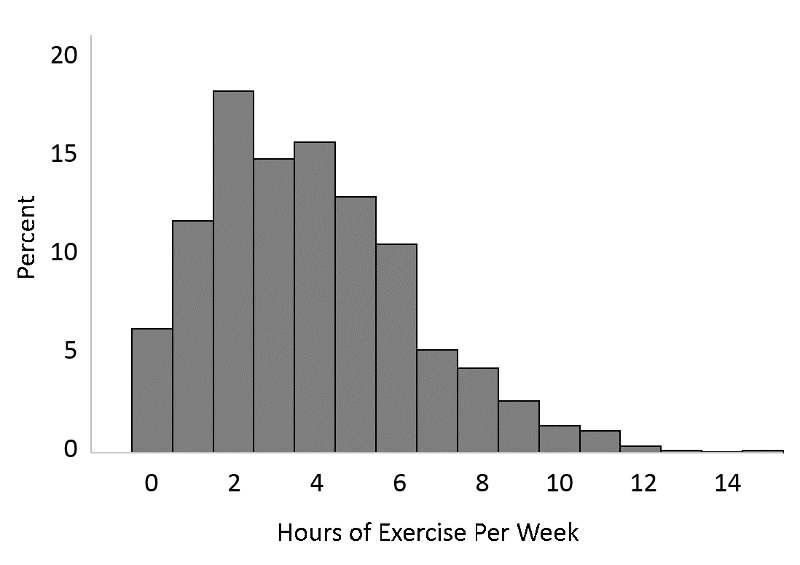
A histogram could be used for continuous variables, and it could also be used for the number of hours of exercise per week which one might think of as an ordinal variable, i.e., discrete, but ordered.
A box and whisker plot is a way of summarizing skewed data. It gives a sense of the shape of the distribution, the central tendency, and the degree of variability.
Example of Box and Whisker Plots Used for Comparison:
Carl and Angela work in a computer store and want to compare the number of sales they made for the past 12 months.
In the past 12 months Angela sold
34, 47, 1, 15, 57, 24, 20, 11, 19, 50, 28, 37
(Ordered: 1, 11, 15, 19, 20, 24, 28, 34, 37, 47, 50, 57)
In the past 12 months Carl sold
51, 17, 25, 39, 7, 49, 62, 41, 20, 6, 43, 13.
(Ordered: 6, 7, 13, 17, 20, 25, 39, 41, 43, 49, 51, 62)
After ordering the data, it can be summarized as follows:
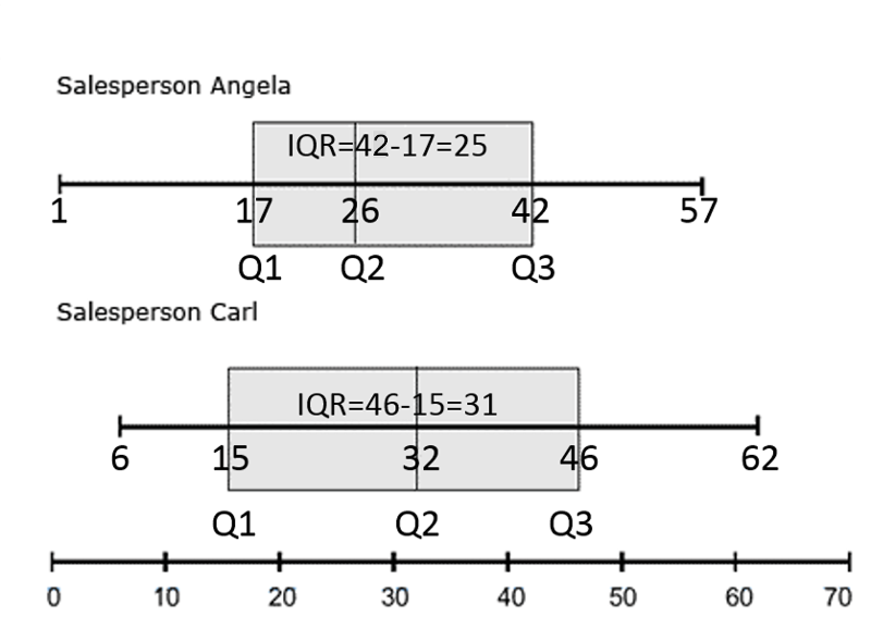
(Image adapted from https://www.statcan.gc.ca/edu/power-pouvoir/ch12/5214889-eng.htm)
Carl's highest and lowest sales are both higher than Angela's, and Carl's median sales figure is higher too. During the past year, Carl consistently sold more computers than Angela.
This course focuses on quantitative methods, which are designed to precisely estimate population parameters and measure the association between biologic, social, environmental, and behavioral factors and health conditions in order to define the determinants of health and disease and, ultimately, to understand causal pathways.
However, it is important to acknowledge the importance of qualitative methods which provide a means of understanding public health problems in greater depth by providing contextual information regarding a population's beliefs, opinions, norms, and behaviors. This type of information is difficult to capture using traditional quantitative methods, yet it can be vitally important for understanding the "why" for many health problems and also the "how" in terms of how to achieve improvements in health outcomes.
These two approaches might be thought of as the positivist and the constructivist approaches. In positivist research data are more easily quantified, but they are disconnected from the context in which they occur. For example, people of lower socioeconomic status are more likely to smoke tobacco, but the data collected does not indicate why. However, with a constructivist approach, the exposures that people are subjected to (or choose) are better understood in the context of their personal circumstances and the significance that people attribute to things in their environment.
Qualitative methods provide a means of understanding health problems and potential barriers and solutions in greater detail, and they provide an opportunity to understand the "how" and "why" and to identify overlooked issues and themes.
The table below, from the introductory course on fundamentals of public health, highlights some of the major differences between quantitative and qualitative research.
| Quantitative | Qualitative | |
|---|---|---|
| General Framework | Test hypotheses; data collection is rigid relying on structured methods, such as questionnaires, surveys, record reviews | Explore phenomena using more flexible methods that categorize responses to semi-structured methods such as in-depth interviews, focus groups, and participant observation |
| Analytic Objectives | Describe populations and to quantify exposure-outcome associations | Describe and explain variations and relationships |
| Question Format | Closed-ended | Open-ended |
| Data Format | Numeric or categorical | Textual (based on audiotapes, videotapes, and field notes) |
| Flexibility in Study Design | Study design is stable throughout a study. Participant responses do not influence or determine how and which questions researchers ask next. | The study design is more flexible. Participant responses affect how and which questions researchers ask next. Questions can be adjusted according to what is learned |


