Part 2 - Introduction to Descriptive Statistics

Population Parameters versus Sample Statistics

A descriptive measure for an entire population is a ''parameter.'' There are many population parameters. For example, the population size (N) is one parameter, and the mean diastolic blood pressure or the mean body weight of a population would be other parameters that relate to continuous variables. Other population parameters focus on discrete variables, such as the percentage of current smokers in the population or the percentage of people with type 2 diabetes mellitus. Health-related behaviors can also be thought of this way, such as the percentage of the population that gets vaccinated against the flu each year or the percentage who routinely wear a seatbelt when driving.

It is generally not feasible to directly measure parameters, since it requires collecting information from all members of the population. We therefore take samples from the population, and the descriptive measures for a sample are referred to as ''sample statistics'' or simply ''statistics.'' For example, the mean diastolic blood pressure, the mean body weight, and the percentage of smokers in a sample from the population would be sample statistics. In the image below the true mean diastolic blood pressure for the population of adults in Massachusetts is 78 millimeters of mercury (mm Hg); this is a population parameter. The image also shows the mean diastolic blood pressure in three separate samples. These means are sample statistics which we might use in order to estimate the parameter for the entire population. However, note that the sample statistics are all a little bit different, and none of them are exactly the sample as the population parameter.

Variables in Public Health

Descriptive statistics are important for monitoring a population (surveillance), for analyzing and communicating trends in both acute and chronic disease frequency and trends in health-related behaviors (e.g., smoking, exercise, alcohol and drug use, seatbelt use, etc.) and many other relevant exposures. Descriptive statistics are also essential for analyzing and communicating the results of descriptive epidemiological studies (case series, cross-sectional studies, and ecologic studies. A variable is anything that has a quantity or quality that varies. We refer to health outcomes and dependent variables , because their occurrence depends on the presence of one or (usually) more than one exposures or risk factors, which are called independent variables. The variables (both exposures and health outcomes) that are collected for these purposes can be of several types.

Variable Types

Categorical variables are those that fall into two or more categories that do not have any inherent ranking or ordering, such as race and ethnicity (e.g., white, black, Hispanic, Asian, etc.)
Dichotomous variables are categorical variables that have just two possible values (e.g., male or female, Occupational exposure to asbestos: Yes or No, Death: Yes or No; developed coronary heart disease: Yes or No)
Ordinal variables are a type of categorical variables that have more than two ranked or ordered values (e.g., physical activity: <30 minutes/week, 30-180 minutes/week, >180 minutes/week; amount of current smoking: none, <10/day, 10-20/day, 21-30/day, >30/day); or number of past heart attacks: 0, 1, 2, 3, etc.)
Continuous (or measurement) variables can assume any numeric value within a specified range (e.g., systolic and diastolic blood pressure in millimeters of mercury, body weight in pound, body mass index, annual income)

Summarizing Dichotomous, Ordinal, and Categorical Variables

Dichotomous, ordinal, and categorical variables are typically summarized by showing the sample size (N), the counts in each group, and the relative frequency or percentage in each group as illustrated by the variables for sex and race/ethnicity in the table below describing some of the baseline characteristics in a randomized clinical trial comparing outcomes in subjects treated with acetaminophen (Tylenol) or ibuprofen.

Variable	Acetaminophen N=150)	Ibuprofen (N=150)
Age in months	40.3 +12.9	39.4 + 13.6
Male sex - no. (%)	86 (57)	93 (62)
Race or ethnic group - no. (%)
White	74 (49)	74 (49)
Black	47 (31)	50 (33)
Hispanic or Latino	35 (33)	37 (25)

Summarizing Continuous Variables

Continuous variables are generally summarized by indicating the number of subjects, an estimate of a central tendency value (a mean or a median ), and an indication of the degree of variability in the measurements ( standard deviation or interquartile range.) In the table below from the same study note that age is reported as mean + standard deviation, because it was a normally distributed continuous variable. IgE antibody levels and eosinophil counts in blood are reported as median and interquartile range because they were not normally distributed.

Variable	Acetaminophen N=150)	Ibuprofen (N=150)
Age in months	40.3 +12.9	39.4 + 13.6
Median IgE (interquartile range - kU/liter	64 (19-176)	70 (24-252)
Median blood eosinophil count (interquartile range) - cells/mm³	259.6 (172.5-534.8	248.4 (132.8-450.0)

Central Tendency Values for Normally Distributed versus Skewed Distributions of Continuous Variables

There are two commonly used methods for describing the central tendency, or most central value of a continuous variable.

The mean is the average value, which is computed by summing the measurements and dividing by the number of observations. For example, suppose seven patients with cardiovascular disease have the following systolic blood pressures:

100 110 114 121 130 130 160

The sum is 865 and the mean is 865/7= 123.6.

The median is the middle value, i.e., the value at which half of the measurements are below that value and half are above. For the small sample of seven subjects above the media systolic blood pressure is 121 mm of mercury since half of the values are below this median and half are above. (To find the median one can sort the values and find the middle value if the number of values is odd; If the number of values is even, the median is the average of the two middle values. However, the R package can do this easily.)

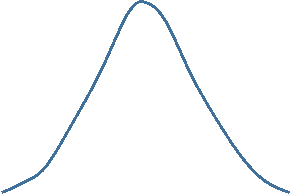
Normal Distributions

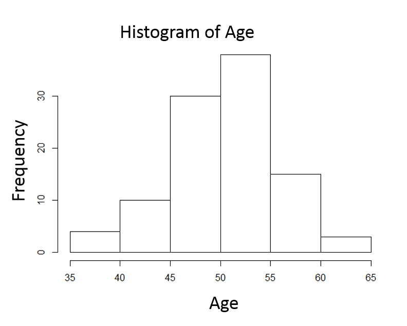
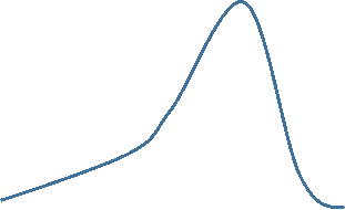
Consider the frequency distribution for the age of landscape workers in the image below.

The frequency distribution of age values is fairly symmetrical with the highest frequencies close to the middle and increasingly less frequent observations moving away from the center in either direction. One might describe the distribution as "bell-shaped," and this is an example of a normal distribution . One typically describes the central tendency with a mean. (Note that the mean and median will be similar in a symmetrical distribution like this.) The mean is calculated by adding all of the values and dividing the sum by the number of observations.

equation image indicator

Variability in a Normal Distribution

For a normal distribution the degree of variability or spread is indicated by the sample variance and the sample standard deviation .

Sample Variance and Sample Standard Deviation:

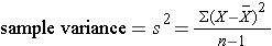
The sample variance is computed by first finding the mean and using it to compute the sum of the squares of the deviation of each value from the mean. The variance is the sum of the squared deviations divided by the sample size minus 1 (i.e., n-1).

equation image indicator


100	-23.6	556.96
110	-13.6	184.96
114	-9.6	92.16
121	-2.6	6.76
130	6.4	40.96
130	6.4	40.96
160	36.4	1324.96
865	0	2247.72

equation image indicator

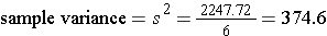
The sample standard deviation is simply the square root of the variance.

equation image indicator

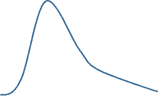
Skewed Distributions or Those with Extreme Outliers

Now consider the frequency distribution of length of stay in the hospital in days as shown below.

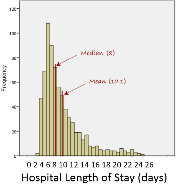
The distribution is not normal; it is skewed to the right . Frequency of length of stay rises to a peak at about 7 days and then very gradually falls with a few patients having stays as long as 24 to 25 days. For a distributed skewed to the right like this the median is a better characterization of the central tendency; the mean is pulled to the right by the extremely long length of stay in small numbers of patients. For skewed distributions like this or distributions with extreme outliers in either direction, one uses the median to characterize the central tendency, and the variability in the observations is described using the interquartile range described below.

Example of the effect of an extreme outlier:

100 110 114 121 130 130 360

This small data set is similar to the one that was previously used except that the last value has been replaced with an "outlier." The median is still 121, but the mean has now been pulled from 123.6 up to 152. So, for data sets with extreme outliers, one should use the median.

Variability in a Skewed Distribution or with Outliers

For clarity, the illustration below of a normal distribution will be used to explain quartiles and interquartile range. However, interquartile range is generally used for data that is not normally distributed.

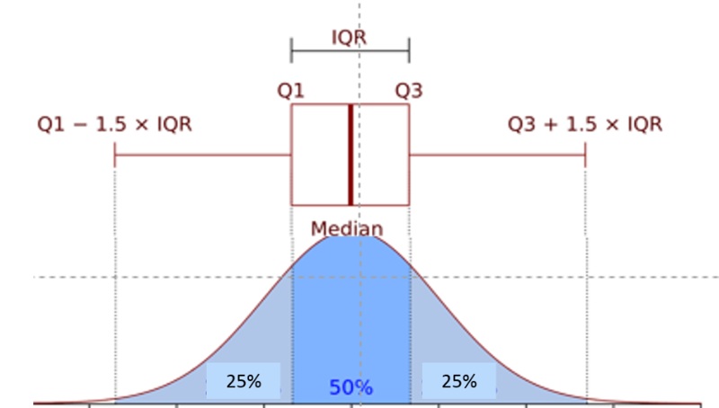
First, the observations are ranked from smallest to greatest, and the data set is divided into four equal parts ( quartiles ) such that each quartile has an equal (or nearly equal) number of observations. Half of the observations will be below the median, and half will be above. The 1^st quartile (Q1) has the lowest 25% of observations, defined by finding the middle value between the lowest and median values. The 4^th quartile (Q4) has the highest 25% of observations and is defined by finding the middle value between the median and the highest value in the data set. The 2^nd quartile (Q2) has the 25% between the 1^st quartile and the median, and the 3^rd quartile (Q3) has the 25% between the median and the 4^th quartile.

The interquartile range (IQR) is the range for the middle 50% of the data, i.e., between Q1 and Q3:

equation image indicator

Example: Consider this small data set:

100, 110, 114, 121, 130, 130, 360

It would be very tedious to compute the IQR by hand, but statistical packages like R make it easy. Here is a preview:

> data<- c(100,110,114,121,130,130,360)

> summary(data)

Min. 1st Qu. Median Mean 3rd Qu. Max.

100.0 112.0 121.0 152.1 130.0 360.0

The lines in blue are commands to R. The first line of code above just creates this small data set, and the second line asks for a summary of the data.

equation image indicator