


Characteristics of Person, Place, and Time
Descriptive epidemiology searches for patterns by examining characteristics of person, place, & time . These characteristics are carefully considered when a disease outbreak occurs, because they provide important clues regarding the source of the outbreak.
Hypotheses about the determinants of disease arise from considering the characteristics of person, place, and time and looking for differences, similarities, and correlations. Consider the following examples:
- Differences : if the frequency of disease differs in two circumstances, it may be caused by a factor that differs between the two circumstances. Example : there was a substantial difference in the incidence of stomach cancer in Japan & the US. Perhaps the difference in incidence of stomach cancer is due to genetic differences or difference in diet.
- Similarities : if a high frequency of disease is found in several different circumstances & one can identify a common factor, then the common factor may be responsible. Example : The occurrence of AIDS in IV drug users, recipients of transfusions, & hemophiliacs suggests the possibility that HIV can be transmitted via blood or blood products.
- Correlations: If the frequency of disease varies in relation to some factor, then that factor may be a cause of the disease. Example: differences in coronary heart disease correlate with cigarettes consumption.
Descriptive epidemiology provides a way of organizing and analyzing data on health and disease in order to understand variations in disease frequency geographically and over time and how disease varies among people based on a host of personal characteristics (person, place, and time). Epidemiology had its origins in the desire to understand the determinants of acute infectious diseases, but its methods and applicability have expanded to include chronic diseases as well.
Person: Personal Characteristics and Behaviors
There are many personal characteristics and behaviors that are relevant to health status and might be considered "exposures" or risk factors that ought to be considered when conducting research on the determinants of disease or when trying to predict risk. Age, sex, and race/ethnicity are almost always variables of potential interest since the frequency of health outcomes can vary markedly with these characteristics. However, one should think broadly about the many other personal characteristics that might be important, such as:
- Occupation
- Diet
- Smoking
- Alcohol consumption
- Medications
- Family history of disease
- Religious practices, e.g. dietary restrictions or restrictions on drinking alcohol or tobacco use
- Leisure activities, e.g., exercise
- Sexual habits
Place: Variation by Location
Where one lives, works, and travels can provide clues about relevant exposures. In addition, surveillance data showing how disease frequency varies geographically, or even within the same workplace, might provide valuable clues about the etiology of a health problem.
- Does the frequency of disease vary from country to country? Or state to state?
- Does it vary among cities or neighborhoods?
- Does it vary within different parts of a large workplace?
Example 1: Stomach Cancer by Location in the US
The maps below show death rates from stomach cancer in females and males in different US counties. The darkness of shading of each county indicates how its stomach cancer rate compares with the national average. The darkest shading indicates rates well above average, and white shading indicates rates below average; the gray shading indicates intermediate levels. Note that rates of stomach cancer tend to be high in counties in the north-central part of the country in both males and females. Investigators speculated that these clusters might correlate with populations of German or Scandinavian descent who have a tradition of eating smoked fish. Could the high rates of stomach cancer be the result of their consumption of smoked fish or other traditional methods of food preservation?
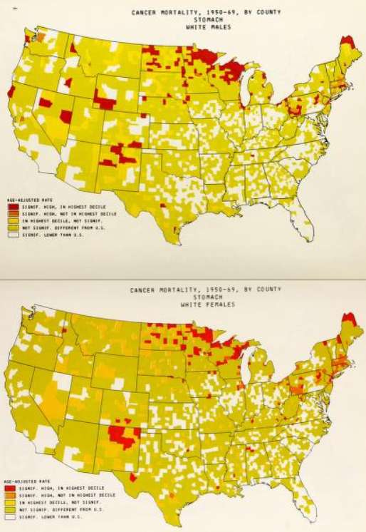
Source: Atlas of Cancer Mortality for U.S. Counties: 1950-1969, TJ Mason et al, PHS, NIH, 1975
https://archive.org/details/atlasofcancermor00nati_0
Example 2: Differences in Rates of Stomach Cancer in Japan and US
Rates of stomach cancer also vary among countries. Japanese have a higher rate of stomach cancer than Caucasians in California. Is this due to a genetic difference? A dietary difference? The rate among Japanese people diminishes after they move to US, and diminishes even more in their offspring. One possibility is that once the Japanese move here, they begin to shift to an American diet, and this trend is even stronger in their children. Are there important dietary differences? Could consumption of large amounts of smoked fish be a cause of stomach cancer?
| Population |
Mortality Rate (per 100,000 population) |
|
Japanese in Japan |
58.4 |
|
Japanese immigrants to California |
29.9 |
|
Sons of Japanese immigrants |
11.7 |
|
Native Californians (Caucasians) |
8.0 |
Variation in Disease Over Time
Public health surveillance systems provide the data to monitor the frequency of health problems over time, and this is vitally important for identifying outbreaks and trends in disease frequency over time. One should consider changes in disease frequency on several different scales depending upon the disease of interest.
- Has the frequency of disease changed over several decades? (e.g., tuberculosis, polio)
- Does frequency of disease vary in a cyclic way that relates to the seasons? (e.g., influenza)
- Has it changed over the course of days? (e.g., outbreaks of foodborne illness)
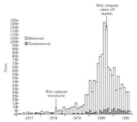
Example: Toxic Shock and Rely Tampons
In January 1980 there were several reports of toxic shock syndrome due to infection with Staphylococcus aureus bacteria, and the descriptive epidemiology indicated that the problem was occurring primarily in menstruating women. A CDC task force investigated and eventually traced the outbreak to the introduction of Rely tampons, a super absorbent product marketed by Proctor and Gamble. The monthly cases of toxic shock syndrome in 1980-1981 are shown in the graph below [from A. Reingold et al., Toxic shock syndrome surveillance in the United States, 1980-1981. Ann. Intern. Med 96:875, 1982]. The graph shows that prior to 1978 there were just occasional cases of toxic shock syndrome in the United States. After Rely tampons were introduced in 1978, there was a steady increase in toxic shock cases which peaked at about 125 per month in 1980. Shortly after that, Rely tampons were taken off the market, and the incidence declined sharply.
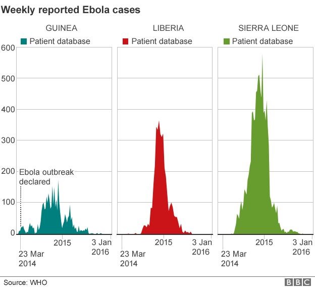
There were also dramatic changes in the frequency of the Ebola epidemic in Africa in 2017, as shown below. The epidemic curves for Guinea, Liberia, and Sierra Leone show that the number of Ebola cases began to rise in March 2014, peaked in mid 2015, and then gradually fell by January 2016.
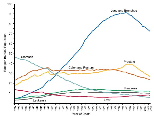
The incidence of some cancers has varied over time as a result of changes in behavior or diagnostic methods and treatment. Decreases in tobacco smoking were followed by a decline in frequency of lung cancer, and modern methods of food preservation led to a decrease in stomach cancer. The diagnosis of prostate cancer increased after introduction of the PSA (prostate specific antigen) test, and mortality from colorectal decreased after the introduction of colonoscopy as a screening and treatment modality. These changes are demonstrated in the graph below, which shows changes in the incidence of selected cancers over time in males.
Other Factors That Can Produce Changes in Disease Frequency Over Years or Decades
- Changes in incidence due to environmental or life-style changes.
- Improvements in diagnosis may increase cases reported even though the incidence may not be changing.
- Changes in record keeping (accuracy) can create what appear to be changes in disease rates.
- Improved treatment may decrease mortality rates
- Changes in the age distribution of a population can produce changes in the overall rate of disease, even if age-specific rates are not changing.