Random Error
At its heart, the goal of an epidemiologic study is to measure a disease frequency or to compare disease frequency in two or more exposure groups in order to measure the extent to which there is an association. There are three primary challenges to achieving an accurate estimate of the association:
Random error occurs because the estimates we produce are based on samples, and samples may not accurately reflect what is really going on in the population at large. .
There are differences of opinion among various disciplines regarding how to conceptualize and evaluate random error. In this module the focus will be on evaluating the precision of the estimates obtained from samples.
After successfully completing this unit, the student will be able to:

Consider two examples in which samples are to be used to estimate some parameter in a population:
The parameters being estimated differed in these two examples. The first was a measurement variable, i.e. body weight, which could have been any one of an infinite number of measurements on a continuous scale. In the second example the marbles were either blue or some other color (i.e., a discrete variable that can only have a limited number of values), and in each sample it was the frequency of blue marbles that was computed in order to estimate the proportion of blue marbles. Nevertheless, while these variables are of different types, they both illustrate the problem of random error when using a sample to estimate a parameter in a population.
The problem of random error also arises in epidemiologic investigations. We noted that basic goals of epidemiologic studies are a) to measure a disease frequency or b) to compare measurements of disease frequency in two exposure groups in order to measure the extent to which there is an association. However, both of these estimates might be inaccurate because of random error. Here are two examples that illustrate this.
Certainly there are a number of factors that might detract from the accuracy of these estimates. There might be systematic error, such as biases or confounding, that could make the estimates inaccurate. However, even if we were to minimize systematic errors, it is possible that the estimates might be inaccurate just based on who happened to end up in our sample. This source of error is referred to as random error or sampling error.
In the bird flu example, we were interested in estimating a proportion in a single group, i.e. the proportion of deaths occurring in humans infected with bird flu. In the tanning study the incidence of skin cancer was measured in two groups, and these were expressed as a ratio in order to estimate the magnitude of association between frequent tanning and skin cancer. When the estimate of interest is a single value (e.g., a proportion in the first example and a risk ratio in the second) it is referred to as a point estimate. For both of these point estimates one can use a confidence interval to indicate its precision.


Strictly speaking, a 95% confidence interval means that if the same population were sampled on infinite occasions and confidence interval estimates were made on each occasion, the resulting intervals would contain the true population parameter in approximately 95% of the cases, assuming that there was no systematic error (bias or confounding). However, because we don't sample the same population or do exactly the same study on numerous (much less infinite) occasions, we need an interpretation of a single confidence interval. The interpretation turns out to be surprisingly complex, but for purposes of our course, we will say that it has the following interpretation: A confidence interval is a range around a point estimate within which the true value is likely to lie with a specified degree of probability, assuming there is no systematic error (bias or confounding). If the sample size is small and subject to more random error, then the estimate will not be as precise, and the confidence interval would be wide, indicating a greater amount of random error. In contrast, with a large sample size, the width of the confidence interval is narrower, indicating less random error and greater precision. One can, therefore, use the width of confidence intervals to indicate the amount of random error in an estimate. The most frequently used confidence intervals specify either 95% or 90% likelihood, although one can calculate intervals for any level between 0-100%. Confidence intervals can also be computed for many point estimates: means, proportions, rates, odds ratios, risk ratios, etc. For this course we will be primarily using 95% confidence intervals for a) a proportion in a single group and b) for estimated measures of association (risk ratios, rate ratios, and odds ratios), which are based on a comparison of two groups.
It is important to note that 95% confidence intervals only address random error, and do not take into account known or unknown biases or confounding, which invariably occur in epidemiologic studies. Consequently, Rothman cautions that it is better to regard confidence intervals as a general guide to the amount of random error in the data. Failure to account for the fact that the confidence interval does not account for systematic error is common and leads to incorrect interpretations of results of studies.
In the example above in which I was interested in estimating the case-fatality rate among humans infected with bird flu, I was dealing with just a single group, i.e., I was not making any comparisons. Lye et al. performed a search of the literature in 2007 and found a total of 170 cases of human bird flu that had been reported in the literature. Among these there had been 92 deaths, meaning that the overall case-fatality rate was 92/170 = 54%. How precise is this estimate?
Link to the article by Lye et al.
There are several methods of computing confidence intervals, and some are more accurate and more versatile than others. The EpiTool.XLS spreadsheet created for this course has a worksheet entitled "CI - One Group" that will calculate confidence intervals for a point estimate in one group. The top part of the worksheet calculates confidence intervals for proportions, such as prevalence or cumulative incidences, and the lower portion will compute confidence intervals for an incidence rate in a single group.
A Quick Video Tour of "Epi_Tools.XLSX" (9:54)
Link to a transcript of the video
Spreadsheets are a valuable professinal tool. To learn more about the basics of using Excel or Numbers for public health applications, see the online learning module on
Link to online learning module on Using Spreadsheets - Excel (PC) and Numbers (Mac & iPad)
Use "Epi_Tools" to compute the 95% confidence interval for the overall case-fatality rate from bird flu reported by Lye et al. (NOTE: You should download the Epi-Tools spreadsheet to your computer; there is also a link to EpiTools under Learn More in the left side navigation of the page.) Open Epi_Tools.XLSX and compute the 95% confidence; then compare your answer to the one below.
ANSWER
How would you interpret this confidence interval in a single sentence? Jot down your interpretation before looking at the answer.
ANSWER
In the hypothetical case series that was described on page two of this module the scenario described 8 human cases of bird flu, and 4 of these died. use Epi_Tools to compute the 95% confidence interval for this proportion. How does this confidence interval compare to the one you computed from the data reported by Lye et al.?
ANSWER
The key to reducing random error is to increase sample size. The table below illustrates this by showing the 95% confidence intervals that would result for point estimates of 30%, 50% and 60%. For each of these, the table shows what the 95% confidence interval would be as the sample size is increased from 10 to 100 or to 1,000. As you can see, the confidence interval narrows substantially as the sample size increases, reflecting less random error and greater precision.
|
Observed Frequency |
Sample Size =10 |
Sample Size =100 |
Sample Size =1000 |
|---|---|---|---|
|
0.30 |
0.11 - 0.60 |
0.22 - 0.40 |
0.27 - 0.33 |
|
0.50 |
0.24 - 0.76 |
0.40 - 0.60 |
0.47 - 0.53 |
|
0.60 |
0.31 - 0.83 |
0.50 - 0.69 |
0.57 - 0.63 |
Video Summary - Confidence Interval for a Proportion in a Single Group (5:11)
Link to transcript of the video
Measures of association are calculated by comparing two groups and computing a risk ratio, a risk difference (or rate ratios and rate differences), or, in the case of a case-control study, an odds ratio. These types of point estimates summarize the magnitude of association with a single number that captures the frequencies in both groups. These point estimates, of course, are also subject to random error, and one can indicate the degree of precision in these estimates by computing confidence intervals for them.
There are several methods for computing confidence intervals for estimated measures of association as well. You will not be responsible for these formulas; they are presented so you can see the components of the confidence interval.

where "RR" is the risk ratio, "a" is the number of events in the exposed group, "N1" in the number of subjects in the exposed group, "c" is the number of events in the unexposed group, and N0 is the number of subjects in the unexposed group.

where IRR is the incidence rate ratio, "a" is the number of events in the exposed group, and"b" is the number of events in the unexposed group.

where "OR" is the odds ratio, "a" is the number of cases in the exposed group, "b" is the number of cases in the unexposed group, "c" is the number of controls in the exposed group, and "d" is the number of controls in the unexposed group.
As noted previously, a 95% confidence interval means that if the same population were sampled on numerous occasions and confidence interval estimates were made on each occasion, the resulting intervals would contain the true population parameter in approximately 95% of the cases, assuming that there were no biases or confounding. However, people generally apply this probability to a single study. Consequently, an odds ratio of 5.2 with a confidence interval of 3.2 to 7.2 suggests that there is a 95% probability that the true odds ratio would be likely to lie in the range 3.2-7.2 assuming there is no bias or confounding. The interpretation of the 95% confidence interval for a risk ratio, a rate ratio, or a risk difference would be similar.
Hypothesis testing (or the determination of statistical significance) remains the dominant approach to evaluating the role of random error, despite the many critiques of its inadequacy over the last two decades. Although it does not have as strong a grip among epidemiologists, it is generally used without exception in other fields of health research. Many epidemiologists that our goal should be estimation rather than testing. According to that view, hypothesis testing is based on a false premise: that the purpose of an observational study is to make a decision (reject or accept) rather than to contribute a certain weight of evidence to the broader research on a particular exposure-disease hypothesis. Furthermore, the idea of cut-off for an association loses all meaning if one takes seriously the caveat that measures of random error do not account for systematic error, so hypothesis testing is based on the fiction that the observed value was measured without bias or confounding, which in fact are present to a greater or lesser extent in every study.
Confidence intervals alone should be sufficient to describe the random error in our data rather than using a cut-off to determine whether or not there is an association. Whether or not one accepts hypothesis testing, it is important to understand it, and so the concept and process is described below, along with some of the common tests used for categorical data.
When groups are compared and found to differ, it is possible that the differences that were observed were just the result of random error or sampling variability. Hypothesis testing involves conducting statistical tests to estimate the probability that the observed differences were simply due to random error. Aschengrau and Seage note that hypothesis testing has three main steps:
1) One specifies "null" and "alternative" hypotheses. The null hypothesis is that the groups do not differ. Other ways of stating the null hypothesis are as follows:

2) One compares the results that were expected under the null hypothesis with the actual observed results to determine whether observed data is consistent with the null hypothesis. This procedure is conducted with one of many statistics tests. The particular statistical test used will depend on the study design, the type of measurements, and whether the data is normally distributed or skewed.
3) A decision is made whether or not to reject the null hypothesis and accept the alternative hypothesis instead. If the probability that the observed differences resulted from sampling variability is very low (typically less than or equal to 5%), then one concludes that the differences were "statistically significant" and this supports the conclusion that there is an association (although one needs to consider bias and confounding before concluding that there is a valid association).
The end result of a statistical test is a "p-value," where "p" indicates probability of observing differences between the groups that large or larger, if the null hypothesis were true. The logic is that if the probability of seeing such a difference as the result of random error is very small (most people use p< 0.05 or 5%), then the groups probably are different. [NOTE: If the p-value is >0.05, it does not mean that you can conclude that the groups are not different; it just means that you do not have sufficient evidence to reject the null hypothesis. Unfortunately, even this distinction is usually lost in practice, and it is very common to see results reported as if there is an association if p<.05 and no association if p>.05. Only in the world of hypothesis testing is a 10-15% probability of the null hypothesis being true (or 85-90% chance of it not being true) considered evidence against an association.]
Most commonly p< 0.05 is the "critical value" or criterion for statistical significance. However, this criterion is arbitrary. A p-value of 0.04 indicates a 4% chance of seeing differences this great due to sampling variability, and a p-value of 0.06 indicates a probability of 6%. While these are not so different, one would be considered statistically significant and the other would not if you rigidly adhered to p=0.05 as the criterion for judging the significance of a result.
Video Summary: Null Hypothesis and P-Values (11:19)
Link to transcript of the video
The chi-square test is a commonly used statistical test when comparing frequencies, e.g., cumulative incidences. For each of the cells in the contingency table one subtracts the expected frequency from the observed frequency, squares the result, and divides by the expected number. Results for the four cells are summed, and the result is the chi-square value. One can use the chi square value to look up in a table the "p-value" or probability of seeing differences this great by chance. For any given chi-square value, the corresponding p-value depends on the number of degrees of freedom. If you have a simple 2x2 table, there is only one degree of freedom. This means that in a 2x2 contingency table, given that the margins are known, knowing the number in one cell is enough to deduce the values in the other cells.
Formula for the chi squared statistic:
One could then look up the corresponding p-value, based on the chi squared value and the degrees of freedom, in a table for the chi squared distribution. Excel spreadsheets and statistical programs have built in functions to find the corresponding p-value from the chi squared distribution.As an example, if a 2x2 contingency table (which has one degree of freedom) produced a chi squared value of 2.24, the p-value would be 0.13, meaning a 13% chance of seeing difference in frequency this larger or larger if the null hypothesis were true.
Chi squared tests can also be done with more than two rows and two columns. In general, the number of degrees of freedom is equal to the number or rows minus one times the number of columns minus one, i.e., degreed of freedom (df) = (r-1)x(c-1). You must specify the degrees of freedom when looking up the p-value.
Using Excel: Excel spreadsheets have built in functions that enable you to calculate p-values using the chi-squared test. The Excel file "Epi_Tools.XLS" has a worksheet that is devoted to the chi-squared test and illustrates how to use Excel for this purpose. Note also that this technique is used in the worksheets that calculate p-values for case-control studies and for cohort type studies.
The chi-square uses a procedure that assumes a fairly large sample size. With small sample sizes the chi-square test generates falsely low p-values that exaggerate the significance of findings. Specifically, when the expected number of observations under the null hypothesis in any cell of the 2x2 table is less than 5, the chi-square test exaggerates significance. When this occurs, Fisher's Exact Test is preferred.
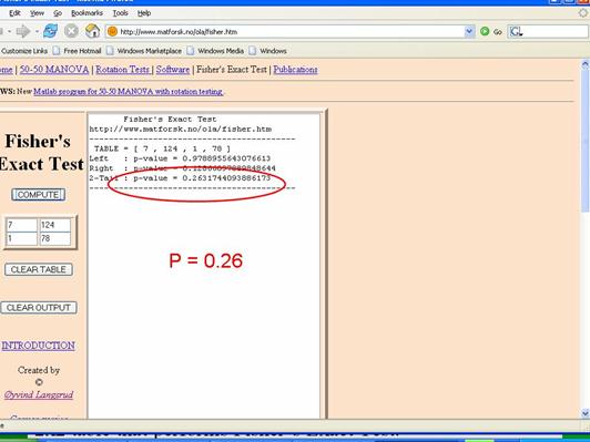
Fisher's Exact Test is based on a large iterative procedure that is unavailable in Excel. However, a very easy to use 2x2 table for Fisher's Exact Test can be accessed on the Internet at http://www.langsrud.com/fisher.htm. The screen shot below illustrates the use of the online Fisher's Exact Test to calculate the p-value for the study on incidental appendectomies and wound infections. When I used a chi-square test for these data (inappropriately), it produced a p-value =0.13. The same data produced p=0.26 when Fisher's Exact Test was used.
Confidence intervals are calculated from the same equations that generate p-values, so, not surprisingly, there is a relationship between the two, and confidence intervals for measures of association are often used to address the question of "statistical significance" even if a p-value is not calculated. We already noted that one way of stating the null hypothesis is to state that a risk ratio or an odds ratio is 1.0. We also noted that the point estimate is the most likely value, based on the observed data, and the 95% confidence interval quantifies the random error associated with our estimate, and it can also be interpreted as the range within which the true value is likely to lie with 95% confidence. This means that values outside the 95% confidence interval are unlikely to be the true value. Therefore, if the null value (RR=1.0 or OR=1.0) is not contained within the 95% confidence interval, then the probability that the null is the true value is less than 5%. Conversely, if the null is contained within the 95% confidence interval, then the null is one of the values that is consistent with the observed data, so the null hypothesis cannot be rejected.
NOTE: Such a usage is unfortunate in my view because it is essentially using a confidence interval to make an accept/reject decision rather than focusing on it as a measure of precision, and it focuses all attention on one side of a two-sided measure (for example, if the upper and lower limits of a confidence interval are .90 and 2.50, there is just as great a chance that the true result is 2.50 as .90).
An easy way to remember the relationship between a 95% confidence interval and a p-value of 0.05 is to think of the confidence interval as arms that "embrace" values that are consistent with the data. If the null value is "embraced", then it is certainly not rejected, i.e. the p-value must be greater than 0.05 (not statistically significant) if the null value is within the interval. However, if the 95% CI excludes the null value, then the null hypothesis has been rejected, and the p-value must be < 0.05.
Video Summary: Confidence Intervals for Risk Ratio, Odds Ratio, and Rate Ratio (8:35)
Link to a transcrip of the video
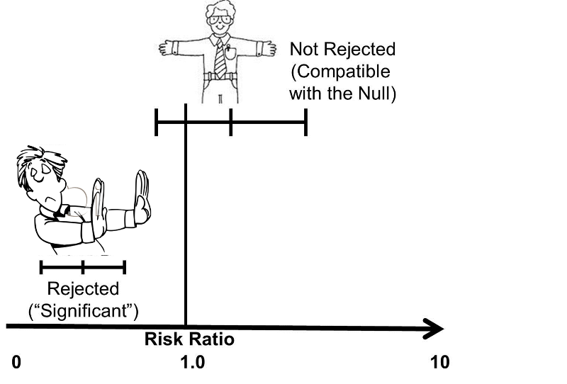
The difference between the perspective provided by the confidence interval and significance testing is particularly clear when considering non-significant results. The image below shows two confidence intervals; neither of them is "statistically significant" using the criterion of P< 0.05, because both of them embrace the null (risk ratio = 1.0). However, one should view these two estimates differently. The estimate with the wide confidence interval was likely obtained with a small sample size and a lot of potential for random error. However, even though it is not statistically significant, the point estimate (i.e., the estimated risk ratio or odds ratio) was somewhere around four, raising the possibility of an important effect. In this case one might want to explore this further by repeating the study with a larger sample size. Repeating the study with a larger sample would certainly not guarantee a statistically significant result, but it would provide a more precise estimate. The other estimate that is depicted is also non-significant, but it is a much narrower, i.e., more precise estimate, and we are confident that the true value is likely to be close to the null value. Even if there were a difference between the groups, it is likely to be a very small difference that may have little if any clinical significance. So, in this case, one would not be inclined to repeat the study.
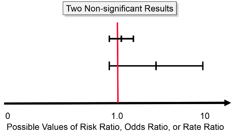
For example, even if a huge study were undertaken that indicated a risk ratio of 1.03 with a 95% confidence interval of 1.02 - 1.04, this would indicate an increase in risk of only 2 - 4%. Even if this were true, it would not be important, and it might very well still be the result of biases or residual confounding. Consequently, the narrow confidence interval provides strong evidence that there is little or no association.
The next figure illustrates two study results that are both statistically significant at P< 0.05, because both confidence intervals lie entirely above the null value (RR or OR = 1). The upper result has a point estimate of about two, and its confidence interval ranges from about 0.5 to 3.0, and the lower result shows a point estimate of about 6 with a confidence interval that ranges from 0.5 to about 12. The narrower, more precise estimate enables us to be confident that there is about a two-fold increase in risk among those who have the exposure of interest. In contrast, the study with the wide confidence interval is "statistically significant," but it leaves us uncertain about the magnitude of the effect. Is the increase in risk relatively modest or is it huge? We just don't know.
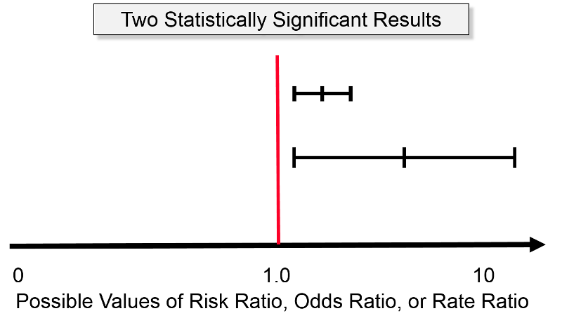
So, regardless of whether a study's results meet the criterion for statistically significance, a more important consideration is the precision of the estimate.
Aschengrau and Seage note that hypothesis testing was developed to facilitate decision making in agricultural experiments, and subsequently became used in the biomedical literature as a means of imposing standards for decision making. P-values have become ubiquitous, but epidemiologists have become increasingly aware of the limitations and abuses of p-values, and while evidence-based decision making is important in public health and in medicine, decisions are rarely made based on the finding of a single study.
Table 12-2 in the textbook by Aschengrau and Seage provides a nice illustration of some of the limitations of p-values.
|
Results of Five Hypothetical Studies on the Risk of Breast Cancer After Childhood Exposure to Tobacco Smoke (Adapted from Table 12-2 in Aschengrau and Seage) |
||||
|---|---|---|---|---|
|
Study |
# Subjects |
Relative Risk |
p value |
"Statistically Significant" |
|
A |
2500 |
1.4 |
0.02 |
Yes |
|
B |
500 |
1.7 |
0.10 |
No |
|
C |
2000 |
1.6 |
0.04 |
Yes |
|
D |
250 |
1.8 |
0.30 |
No |
|
E |
1000 |
1.6 |
0.06 |
No |
The authors start from the assumption that these five hypothetical studies constitute the entire available literature on this subject and that all are free from bias and confounding. The authors point out that the relative risks collectively and consistently suggest a modest increase risk, yet the p-values are inconsistent in that two have "statistically significant" results, but three do not. In this example, the measure of association gives the most accurate picture of the most likely relationship. The p-value is more a measure of the "stability" of the results, and in this case, in which the magnitude of association is similar among the studies, the larger studies provide greater stability.
Video: Just For Fun: What the p-value?
NOTE: This section is optional; you will not be tested on this
Rather than just testing the null hypothesis and using p<0.05 as a rigid criterion for statistically significance, one could potentially calculate p-values for a range of other hypotheses. In essence, the figure at the right does this for the results of the study looking at the association between incidental appendectomy and risk of post-operative wound infections. This study enrolled 210 subjects and found a risk ratio of 4.2. The chi-square test gave a p-value of 0.13, and Fisher's Exact Test gave a p-value of 0.26, which are "not statistically significant." However, to many people this implies no relationship between exposure and outcome.
The graph below gives a more complete summary of the statistical relationship between exposure and outcome. The peak of the curve shows the RR=4.2 (the point estimate). In a sense this point at the peak is testing the null hypothesis that the RR=4.2, and the observed data have a point estimate of 4.2, so the data are VERY compatible with this null hypothesis, and the p-value is 1.0. As you move along the horizontal axis, the curve summarizes the statistical relationship between exposure and outcome for an infinite number of hypotheses.
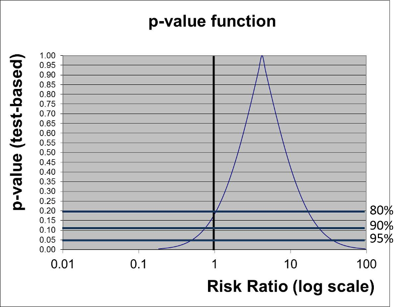
The three horizontal blue lines labeled 80%, 90%, and 95% each intersect the curve at two points which indicate the arbitrary 80, 90, and 95% confidence limits of the point estimate. If we consider the null hypothesis that RR=1 and focus on the horizontal line indicating 95% confidence (i.e., a p-value= 0.05), we can see that the null value is contained within the confidence interval. Note also that the curve intersects the vertical line for the null hypothesis RR=1 at a p-value of about 0.13 (which was the p-value obtained from the chi-square test).
However, if we focus on the horizontal line labeled 80%, we can see that the null value is outside the curve at this point. In other words, we are 80% confident that the true risk ratio is in the range of RR from 1 to about 25.
We noted above that p-values depend upon both the magnitude of association and the precision of the estimate (based on the sample size), but the p-value by itself doesn't convey a sense of these components individually; to do this you need both the point estimate and the spread of the confidence interval. The p-value function above does an elegant job of summarizing the statistical relationship between exposure and outcome, but it isn't necessary to do this to give a clear picture of the relationship. Reporting a 90 or 95% confidence interval is probably the best way to summarize the data.