SAS Basics - Part 1
This module will introduce some basic, but very important and frequently used commands and operations in SAS.
After completing this modules, the student will be able to:
The general format of a data step is as follows:
data name1;
input varl var2 $ var3;
<Programming Statements>;
datalines;
<Data Matrix>
;
run;
Line 1: In the first line we designate a name for the new data set. Here the data set is called name1. The data set name may be up to 32 alphanumeric characters and must begin with a letter. No special characters are allowed in the name except for '_'.
Line 2: The input statement indicates which variables are included in the data set. Here there are 3 variables with the names: var1, var2, var3. SAS differentiates between variables whose values are numeric and variables whose values are character. For character variables, a dollar sign '$' must be added after the name of the variable (like for var2 above). The variable names may be up to 32 alphanumeric characters and must begin with a letter. No special characters are allowed in the variable name except for '_'.
Line 3: There may be many lines of programming statements between the input statement and the datalines statement. Programming statements are used to manipulate the variables in the data set, create new variables, label and format variables, and exclude observations from the data set.
Line 4: Tells SAS that the data to be analyzed are next. Note that cards may be used instead of datalines.
Line 5: The data matrix contain rows of observations and columns of variables.
Line 6: The final semicolon indicates that there is no more data to be read.
Line 7: The run; statement must be on the last line of the data step and indicates that the data step is finished.
Example:
In module 1 we created a very small data set in SAS as follows:
data weight;
input height weight;
cards;
65 130
70 150
67 145
72 180
62 110
;
run;
"Proc" statements are the procedures that are to be performed on the data set.
General Format:
proc <procedure name> data =<data set name> <options>;
<SAS statements>;
run;
"proc print" is the procedure that lists data:
proc print data=name <options>;
var varl var2;
run;
Example:
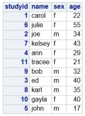
First the data set is defined and the data ("cards") are input.
data one;
input studyid name $ sex $ age weight height;
cards;
run;
[The next steps in the program are commands to print the specified fields in the data set.]
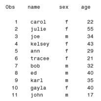
proc print data=one;
var name sex age;
run;
Here is the resulting output:
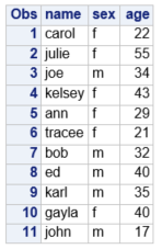
Notice that, by default, SAS adds a variable OBS in the output for proc print that indexes the rows in the data set. However, the noobs option can be used to suppress OBS from the Output.
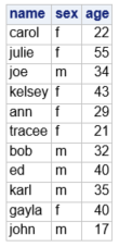
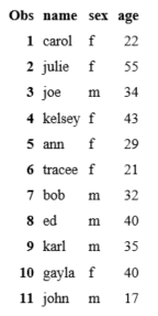
proc print data=one noobs;
var name sex age;
run;
Alternatively, a variable can be substituted for the obs column using the id command.
proc print data=one;
var name sex age;
id studyid;
run;
The id statement in proc print is helpful when printing so many variables that the output does not fit on one page. Using the id statement will ensure that the id variable specified is on each page of the output.
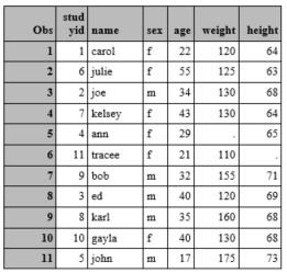
The output shown in the original example above is what you see in the results window. The output in the output window looks like this:
If you want to copy output from SAS to paste into a Word document, you can select and copy from the results window. This will look like this:
In a later lecture, we will show you how to extract the results so they look as nice as they do in the results window!
Note that the var statement is not required. If it is omitted, SAS will, by default, print all the variables in the data set.
proc print data=one;
run;
proc means produces descriptive statistics on continuous variables: mean, standard deviation, etc.
proc means data=name <options>;
var varl var2;
run;
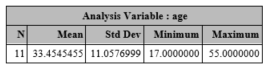
Example:
proc means data=one;
var age;
run;
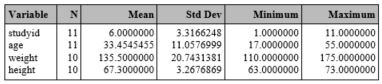
Again, if we omit the var statement, SAS will provide results for all (continuous) variables.
proc means data=one;
run;
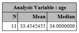
We can also select specific statistics to be calculated and displayed. These include the default statistics, N, Mean, Std, Min, Max, and others, such as Median, Q1, and Q3. Here, we ask for just N, Mean and Median to be displayed :
proc means data=one n mean median;
var age;
run;
SAS datasets can be temporary or permanent.
Unless otherwise specified to be permanent, SAS considers all datasets to be temporary.
SAS calls the directories that contain datasets libraries. To create a library, use a libname statement. A libname statement performs 2 important tasks:
Once a SAS library and computer directory link have been created using the libname statement, a permanent SAS data set can be:
|
A SAS data set name has the library name before the period and the data set name after the period. For example, lib.ds indicates that data set ds is in library lib. In the directory linked to the library lib, there will be a (permanent) data set called ds.sas7bdat. [The extension sas7bdat is just a convention that SAS uses for permanent data sets.] |
Example:
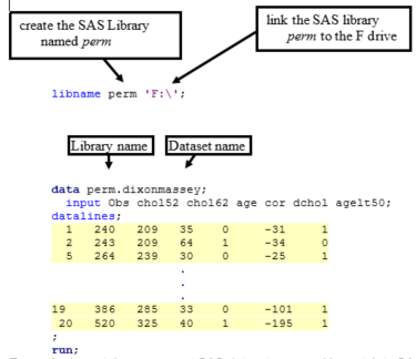
Note: The 'dixonmassey' data set is from Dixon WJ and Massey FJ Jr: Introduction to Statistical Analysis, Fourth Edition, McGraw Hill Book Company, 1983.
Use a libname statement to establish the library perm and to link it to the F drive. Then save the data set dixonmassey as a permanent SAS data set on the F drive. The statement data perm.dixonmassey creates a SAS data set called "dixonmassey.sas7bdat" located in the F drive.
The statement below creates a SAS library named "perm" and then links "perm" to the F drive.
libname perm 'F:\';
The next statement calls from the library called "perm" and selects the data set called "dixonmassey."
Example:
Import the permanent SAS data set, copy_cd4count, into SAS.
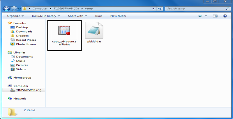
The libname statement below creates a SAS library named extern and links the library extern to the directory "C:\temp" on the computer. The data set copy_cd4count.sas7bdat which is stored in the directory "C:\temp", is now in the extern SAS library and can be used immediately in SAS data steps and procedures. Note that once it has been linked to the extern SAS library, it does not need the extension .sas7bdat.
libname extern 'C:\temp';
proc means data=extern.copy_cd4cout;
run;
When a library is not specified, SAS automatically uses the temporary library "work."
data dixonmassey;
input Obs chol52 chol62 age cor dchol agelt50;
datalines;
…
;
run;
[Note: The "dixonmmassey" data set is from Dixon WJ and Massey FJ Jr., Introduction to Statistical Analysis, Fourth Edition, McGraw Hill Book Company, 1983. ]
SAS interprets the first data line as data WORK.dixonmassey;
In the log, the following NOTE will appear:
NOTE: The data set WORK.DIXONMASSEY has 20 observations and 7 variables.
Remember that the work library is only temporary and when SAS is closed all of the datasets in work are deleted.
Suppose we have a data set called weight which has height and weight data.
data weight;
input height weight;
cards;
65 130
70 150
67 145
72 180
62 110
;
run;
We would like to create a new data set with a new variable, BMI, or body mass index, based on height and weight.
To create a new variable choose a name for the new variable, use a data step, and then define it based on already existing variables using the equals sign (=).
Examples
Body mass index (BMI) is equal to (weight in pounds x 703) / (height in inches)2
So in this case, if we had a data set that contained weight in pounds and height in inches, we could use SAS to compute a derived variable called "bmi" based on these two other variables. Here's how we can do this in SAS:
data w;
input height weight;
bmi = (weight*703)/(height**2);
cards;
65 130
70 150
67 145
72 180
62 110
;
run;
The data set "w" has three variables, height, weight, and bmi. Note that the statement creating the new variable, bmi, is between the input statement and the cards statement. The creation of a new variable always occurs within a data step.
|
Note: The creation of a new variable always occurs within a data step. |
It is also possible to take an existing data set and create a new data set with additional variables, instead of inputting the data anew. We first create a copy of the data set using the set statement, and then make changes in the data step. The following data step creates a SAS data set called weight_new, which is identical to the SAS data set weight.
data weight_new;
set weight;
run;
The set statement puts the data from the data set weight (created above) into a new data set called weight_new. Because the data set weight already exists within SAS, no input statement is necessary. Note that the structure and contents of the new data set weight_new are identical to those of the SAS data set weight.
You can look at your log file to confirm what your code is doing:
92 data weight_new;
93 set weight;
94 run;
NOTE: There were 5 observations read from the data set WORK.WEIGHT.
NOTE: The data set WORK.WEIGHT_NEW has 5 observations and 2 variables.
The log will always show you your code and then log notes (and warnings and errors). From now on, we will only show the actual log (not the code).
In order to create a new variable in an existing SAS data set, the data set must first be read into SAS and then a data step must be used to create a new SAS data set and the new variable.
The following data step creates a new (temporary) SAS data set called bmidata, which is identical to the SAS data set weight but with the addition of a new variable bmi.
data bmidata1;
set weight;
bmi = (weight*703)/(height**2);
run;
NOTE: There were 5 observations read from the data set WORK.WEIGHT.
NOTE: The data set WORK.BMIDATA1 has 5 observations and 3 variables.
We can also create a new data set from an already existing permanent SAS data set. We first import the permanent SAS data set in the C: directory called weight.sas7bdat,and create a new (temporary) SAS data set called bmidata2, with the addition of the variable bmi.
libname indata 'C:\Users';
data bmidata2;
set indata.weight;
bmi = (weight*703)/(height**2);
run;
NOTE: There were 5 observations read from the data set INDATA.WEIGHT.
NOTE: The data set WORK.BMIDATA2 has 5 observations and 3 variables.
Next, we will import the permanent SAS data set weight.sas7bdat in the C: directory and create a new permanent SAS data set in the C: directory called weight1.sas7bdat, again adding the variable bmi. Note that we do not have to include the libname statement again since we have already done so above (in the same SAS session).
data indata.weight1;
set indata.weight;
bmi = (weight*703)/(height**2);
run;
NOTE: There were 5 observations read from the data set INDATA.WEIGHT.
NOTE: The data set INDATA.WEIGHT1 has 5 observations and 3 variables.
An if-then statement can be used to create a new variable for a selected subset of the observations.
For each observation in the data set, SAS evaluates the expression following the if. When the expression is true, the statement following then is executed.
Example:
if age ge 65 then older=1;
When the expression is false, SAS ignores the statement following then. For a person whose age is less than 65, the variable older will be missing.
Note that the above statement could equivalently be written
if age >= 65 then older=1;
An optional else statement can be included (if-then-else) to provide an alternative action when the if expression is false.
if age ge 65 then older=1;
else older=0;
For a person whose age is less than 65, the variable older will equal 0.
An optional else-if statement can follow the if-then statement. SAS evaluates the expression in the else-if statement only when the previous expression is false. else-if statements are useful when forming mutually exclusive groups.
if 40 < age <= 50 then agegroup=1;
else if 50 < age <= 60 then agegroup=2;
else if age > 60 then agegroup=3;
Note that this if-then-else-if statement could equivalently be written
if 40 lt age le 50 then agegroup=1;
else if 50 lt age le 60 then agegroup=2;
else if age gt 60 then agegroup=3;
An if statement can be followed by exactly one else statement or by many else-if statements. SAS will keep evaluating the if-then-else-if statements until it encounters the first true statement.
|
Character variable data must always be enclosed in quotes.
|
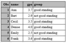
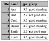
The following code creates a new variable called group from an existing variable called gpa. The new variable called group takes on one of two values: "good standing" if a person's gpa is greater than or equal to 3.0 and "not good standing" if a person's gpa is less than 3.0.
data grades;
input name $ gpa;
if gpa<3.0 then group = "not good standing";
if gpa>=3.0 then group = "good standing";
cards;
Ann 3.7
Bart 2.9
Cecil 3.5
Denise 4.0
Emily 2.5
Frank 3.6
;
run;
proc print;
run;
This results in:
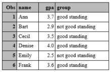
Note that SAS does not generally distinguish between upper and lower case (you can use either). The exception is in the value of character variables. The value "Good standing" is not the same as the value "good standing".
|
SAS code follows the rules of logic: SAS evaluates if-then statements in the order in which they appear in the datastep. |
Suppose we want to create a variable called gpagroup which takes on one of 3 values:
We run the following code:
data grades;
input name $ gpa;
if gpa>=3.5 then gpagroup = "Excellent Grades";
if gpa>=3.0 then gpagroup = "Good";
if gpa >= 2.5 then gpagroup = "Satisfactory";
cards;
Ann 3.7
Bart 2.9
Cecil 3.5
Denise 4.0
Emily 2.5
Frank 3.6
;
run;
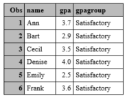
 What went wrong?
Answer
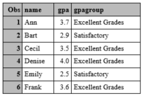
We should instead use if-then-else statements as follows:
data grades;
input name $ gpa;
if gpa>=3.5 then gpagroup = "Excellent Grades";
else if gpa>=3.0 then gpagroup = "Good";
else if gpa >= 2.5 then gpagroup = "Satisfactory";
cards;
Ann 3.7
Bart 2.9
Cecil 3.5
Denise 4.0
Emily 2.5
Frank 3.6
;
run;
proc print;
run;
Suppose we have collected the following data on the ages of 5 people:
id age
1 35
2 missing
3 24
4 38
5 29
Individual 2 has a missing age value, so the data would be entered as follows:
data ages;
input id age;
cards;
1 35
2 .
3 24
4 38
5 29
;
run;
If we run proc means, we would get the following:
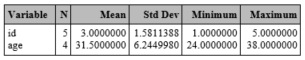
SAS will automatically exclude missing values from calculations, if they are coded correctly. Notice that N=4 for the age variable, because there are only 4 observations with non-missing ages.
However, some data sources will code missing values as 9 or -9 or 99, or some other numeric value. If this is the case, you should immediately re-code these to periods. If you don't recode the missing values, here is what will happen:
Example:
data ages;
input id age;
cards;
1 35
2 -9
3 24
4 38
5 29
;
run;
If we run proc means, we would get the following:
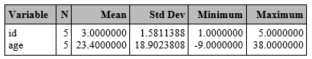
Notice that the minimum age is negative! And the mean age is less than the youngest age in the data set.
|
Important: Always check output for results that make no sense. |
If a data set has missing values coded as anything other than a period, you need to convert these before running the SAS program. This can be done easily by adding an if statement to the data step as illustrated in the example below.
data ages;
input id age;
if age eq -9 then age=.;
cards;
1 35
2 -9
3 24
4 38
5 29
;
run;
If we run proc means, we would get the following:
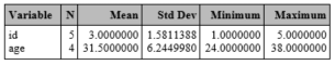
The observation with missing age coded as -9, now has age coded correctly with a period. Notice that the minimum age is now (correctly) 24, and that the mean is actually in the range of the ages! Also notice that N=4 for the age variable, because there are only 4 observations with non-missing ages.
Now we will create a variable called agecat which takes on the value of 1 if the age is less than or equal to 30 and 2 if the age is greater than 30.
We have checked (how?) and the missing age has been correctly coded.
data ages;
input id age;
if age<=30 then agecat = 1;
else if age>30 then agecat=2;
cards;
1 35
2 .
3 24
4 38
5 29
;
run;
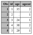
What is wrong with this?
The 2nd observation had a missing age value but was categorized as "young". This person should have a missing age category!
The problem here is that SAS treats missing numeric values as negative infinity. Here, SAS treats the missing age value as negative infinity, which is definitely less than 30, so this observation will be assigned agecat=1.
To fix this problem we need to recode the agecat variable to specifically account for missing values:
data ages;
input id age;
if age = . then agecat = .;
else if age<=30 then agecat = 1;
else if age>30 then agecat=2;
cards;
1 35
2 .
3 24
4 38
5 29
;
run;
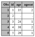
Now the observation with missing age also has a missing agecat variable.
|
Variable |
N |
Mean |
Std Dev |
Minimum |
Maximum |
|
id |
5 |
3.0000000 |
1.5811388 |
1.0000000 |
5.0000000 |
|
age |
4 |
32.5000000 |
6.2449980 |
24.0000000 |
38.0000000 |
|
agecat |
4 |
1.5000000 |
0.5773503 |
1.0000000 |
2.0000000 |
If your data had missing age coded as -9, you would first have to re-code missing age to a period, and then account for missing ages in creating agecat.
data ages;
input id age;
if age eq -9 then age=.;
if age = . then agecat = .;
else if age<=30 then agecat = 1;
else if age>30 then agecat=2;
cards;
1 35
2 -9
3 24
4 38
5 29
run;
Consider the following data step:
data region;
input urban_area $;
cards;
Atlanta
Boston
Los_Angeles
Seattle
Washington_DC
;
run;
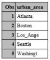
What looks wrong here?
In printing these data, the value of the variable urban_data has been cut off. To prevent this, you must use a length statement when creating character variables.
data region;
length urban_area $13;
input urban_area $;
cards;
Atlanta
Boston
Los_Angeles
Seattle
Washington_DC
;
run;
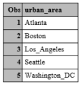
The length statement specifies the maximum length for the values of a variable. The length statement should come at the beginning of the data step, before the variables for which the lengths are being set are defined.
This is true for variables entered using an input statement, or those created in a data step.
Recall the example in which we categorized grades into group;
data grades;
input name $ gpa;
if gpa<3.0 then group = "not good standing";
if gpa>=3.0 then group = "good standing";
cards;
Ann 3.7
Bart 2.9
Cecil 3.5
Denise 4.0
Emily 2.5
Frank 3.6
;
run;
proc print;
run;
Why were the character variable values not truncated?
SAS will use the first value it encounters if there is no length statement. So, in the example, the first value is "not good standing," and so the length is set at 17, which is more than enough for the value "good standing".
If we had instead reversed the two lines of code, the length of the variable group would be set to 13, and some of the values would be truncated.
data grades;
input name $ gpa;
if gpa>=3.0 then group = "good standing";
if gpa<3.0 then group = "not good standing";
cards;
Ann 3.7
Bart 2.9
Cecil 3.5
Denise 4.0
Emily 2.5
Frank 3.6
;
run;
If you are accessing an already created SAS data set (temporary or permanent), you do not have to use a length statement, as the length is stored with the SAS data set.
|
Note: Output can build up in the Results Viewer and you cannot clear it as you can the output window. To clear the Results Viewer, use the following two ODS statements. The first closes the viewer and the second opens it, clearing it as it opens.
ods html close; ods html; run; |
In order to understand how to create new variables using mathematical expressions in SAS we must first review the rules of operation:
Rule 1: Expressions within parentheses are evaluated first.
Rule 2: Operations are performed in order of priority.
= or eq (equal)
^= or ne (not equal)
> or gt (greater than)
< or lt (less than)
>= or ge (greater than or equal to)
<= or le (less than or equal to)
^ or not (negation)
Rule 3: For operators with the same priority, operations are performed left to right except for priority 1 operations which are performed right to left.
Example 1:
. B = 3, C = 6, D = 9
X = B * C / D
= 3 * 6 / 9
= 18 / 9
= 2
Example 2:
G = 2, H = 4, I = 1, J = 3
X = G / I + H * J
= 2 / 1 + 4 * 3
= 2 + 4 * 3
= 2 + 12
= 14
Example 3:
Y = 2, Z = 3, A = 2
X = Y * Z**A
= 2 * 3**2
= 2 * 9
= 18
Calculates the sum of the variables in parentheses. Missing values are treated as 0.
sum(var1, var2, var3)
Finds the average of the variables in parentheses. If a value is missing for a given observation, then the average of the non-missing variables is calculated.
mean(var1, var2, var3, var4)
sqrt(var)
log(var)
Example:
We have data on brain MRI measures in six people, one measure of total cranial volume (TCV), which should not change much over time, and three measures of total brain volume (TCB).
We want to look at change in TCBV, the ratio of TCB to TCV from time 1 to time 2. We do this in two ways. First we calculate TCBV at each time, and simply subtract these two variables. We also do this in one statement (without first calculating the two TCBV variables).
Next we create a new variable which is the log of this difference.
Finally, we want to create the average TCB over the three measures (and try three different methods).
data one;
input id tcb1 tcb2 tcb3 tcv;
tcbv1=tcb1/tcv;
tcbv2=tcb2/tcv;
tcbv_d_A=(tcb1/tcv)-(tcb2/tcv);
tcbv_d_B=tcbv1-tcbv2;
log_d=log(tcbv_d_A);
mean_tcb=mean(of tcb1,tcb2,tcb3);
ave_tcb_A=(tcb1+tcb2+tcb3)/3;
ave_tcb_B=tcb1+tcb2+tcb3/3;
cards;
1 980 975 975 1255
2 994 980 970 1262
3 1015 1002 1000 1280
4 940 . 900 1240
5 1020 1010 . 1259
6 998 998 990 1245
Let's look at the log.
689 data one;
690 input id tcb1 tcb2 tcb3 tcv;
691 tcbv1=tcb1/tcv;
692 tcbv2=tcb2/tcv;
693 tcbv_d_A=(tcb1/tcv)-(tcb2/tcv);
694 tcbv_d_B=tcbv1-tcbv2;
695 log_d=log(tcbv_d_A);
696 mean_tcb=mean(of tcb1,tcb2,tcb3);
697 ave_tcb_A=(tcb1+tcb2+tcb3)/3;
698 ave_tcb_B=tcb1+tcb2+tcb3/3;
699 cards;
NOTE: Invalid argument to function LOG(0) at line 695 column 9.
RULE: ----+----1----+----2----+----3----+----4----+----5----+----6----+----7----+----8----+---
705 6 998 998 990 1245
id=6 tcb1=998 tcb2=998 tcb3=990 tcv=1245 tcbv1=0.8016064257 tcbv2=0.8016064257 tcbv_d_A=0
tcbv_d_B=0 log_d=. mean_tcb=995.33333333 ave_tcb_A=995.33333333 ave_tcb_B=2326 _ERROR_=1 _N_=6
NOTE: Missing values were generated as a result of performing an operation on missing values.
Each place is given by: (Number of times) at (Line):(Column).
1 at 692:13 1 at 693:28 1 at 694:17 1 at 695:9 1 at 697:18 1 at 697:23
1 at 698:17 1 at 698:27
NOTE: Mathematical operations could not be performed at the following places. The results of the
operations have been set to missing values.
Each place is given by: (Number of times) at (Line):(Column).
1 at 695:9
NOTE: The data set WORK.ONE has 6 observations and 13 variables.
Since for ID 6, the difference between TCBV at times 1 and 2 is zero, the log of this difference cannot be calculated, and SAS tells you this, and sets log_d to missing.
Notice that tcbv_d_A and tcbv_d_B are exactly the same.
Which of the three average calculations is correct?