Correlation and Regression with R

Table of Contents»

Contributing Authors:

Ching-Ti Liu, PhD, Associate Professor, Biostatistics

Jacqueline Milton, PhD, Clinical Assistant Professor, Biostatistics

Avery McIntosh, doctoral candidate

This module will provide you with skills that will enable you to perform:

Simple regression and correlation
Multiple regression
Regression diagnostics

Learning Objectives

By the end of this session students will be able to:

Explain concepts of correlation and simple linear regression
Perform correlation and regression analysis using R
Interpret results from correlation and regression
Perform residual analysis to check the assumptions of regression

The Dataset

The dataset we will use here is Penrose et al. (1985). This dataset contains 252 observations and 19 variables, and is described below. First we need to load the data.

> fat <- read.table("fatdata.txt",header=TRUE, sep="\t")

> str(fat)

Table 1. Description of Percent Body Fat data

Variable	Description
id	Case Number
pctfat.brozek	Percent body fat using Brozek's equation, 457/Density - 414.2
pctfat.siri	Percent body fat using Siri's equation, 495/Density - 450
density	Density (gm/cm^3)
age	Age (yrs)
weight	Weight (lbs)
height	Height (inches)
adiposity	Adiposity index = Weight/Height^2 (kg/m^2)
fatfreeweight	Fat Free Weight = (1 - fraction of body fat) * Weight, using Brozek's formula (lbs)
neck	Neck circumference (cm)
chest	Chest circumference (cm)
abdomen	Abdomen circumference (cm) "at the umbilicus and level with the iliac crest"
hip	Hip circumference (cm)
thigh	Thigh circumference (cm)
knee	Knee circumference (cm)
ankle	Ankle circumference (cm)
biceps	Extended biceps circumference (cm)
forearm	Forearm circumference (cm)
wrist	Wrist circumference (cm) "distal to the styloid processes"

The percentage of body fat is a measure to assess a person's health and is measured through an underwater weighing technique. In this lecture we will try to build a formula to predict an individual's body fat, based on variables in the dataset.

Correlation

Correlation is one of the most common statistics. Using one single value, it describes the "degree of relationship" between two variables. Correlation ranges from -1 to +1. Negative values of correlation indicate that as one variable increases the other variable decreases. Positive values of correlation indicate that as one variable increase the other variable increases as well. There are three options to calculate correlation in R, and we will introduce two of them below.

For a nice synopsis of correlation, see https://statistics.laerd.com/statistical-guides/pearson-correlation-coefficient-statistical-guide.php

Pearson Correlation

The most commonly used type of correlation is Pearson correlation, named after Karl Pearson, introduced this statistic around the turn of the 20^th century. Pearson's r measures the linear relationship between two variables, say X and Y. A correlation of 1 indicates the data points perfectly lie on a line for which Y increases as X increases. A value of -1 also implies the data points lie on a line; however, Y decreases as X increases. The formula for r is

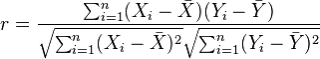
(in the same way that we distinguish between Ȳ and µ, similarly we distinguish r from ρ)

The Pearson correlation has two assumptions:

The two variables are normally distributed. We can test this assumption using

A statistical test (Shapiro-Wilk)
A histogram
A QQ plot

The relationship between the two variables is linear. If this relationship is found to be curved, etc. we need to use another correlation test. We can test this assumption by examining the scatterplot between the two variables.

To calculate Pearson correlation, we can use the cor() function. The default method for cor() is the Pearson correlation. Getting a correlation is generally only half the story, and you may want to know if the relationship is statistically significantly different from 0.

H₀: There is no correlation between the two variables: ρ = 0
H_a: There is a nonzero correlation between the two variables: ρ ≠ 0

To assess statistical significance, you can use cor.test() function.

> cor(fat$age, fat$pctfat.brozek, method="pearson")

[1] 0.2891735

> cor.test(fat$age, fat$pctfat.brozek, method="pearson")

Pearson's product-moment correlation

data: fat$age and fat$pctfat.brozek

t = 4.7763, df = 250, p-value = 3.045e-06

alternative hypothesis: true correlation is not equal to 0

95 percent confidence interval:

0.1717375 0.3985061

sample estimates:

cor

0.2891735

When testing the null hypothesis that there is no correlation between age and Brozek percent body fat, we reject the null hypothesis (r = 0.289, t = 4.77, with 250 degrees of freedom, and a p-value = 3.045e-06). As age increases so does Brozek percent body fat. The 95% confidence interval for the correlation between age and Brozek percent body fat is (0.17, 0.40). Note that this 95% confidence interval does not contain 0, which is consistent with our decision to reject the null hypothesis.

Spearman's rank correlation

Spearman's rank correlation is a nonparametric measure of the correlation that uses the rank of observations in its calculation, rather than the original numeric values. It measures the monotonic relationship between two variables X and Y. That is, if Y tends to increase as X increases, the Spearman correlation coefficient is positive. If Y tends to decrease as X increases, the Spearman correlation coefficient is negative. A value of zero indicates that there is no tendency for Y to either increase or decrease when X increases. The Spearman correlation measurement makes no assumptions about the distribution of the data.

The formula for Spearman's correlation ρ_s is

where d_i is the difference in the ranked observations from each group, (x_i – y_i), and n is the sample size. No need to memorize this formula!

> cor(fat$age,fat$pctfat.brozek, method="spearman")

[1] 0.2733830

> cor.test(fat$age,fat$pctfat.brozek, method="spearman")

Spearman's rank correlation rho

data: fat$age and fat$pctfat.brozek

S = 1937979, p-value = 1.071e-05

alternative hypothesis: true rho is not equal to 0

sample estimates:

rho

0.2733830

Thus we reject the null hypothesis that there is no (Spearman) correlation between age and Brozek percent fat (r = 0.27, p-value = 1.07e-05). As age increases so does percent body fat.

Some Notes on Correlation

Correlation, useful though it is, is one of the most misused statistics in all of science. People always seem to want a simple number describing a relationship. Yet data very, very rarely obey this imperative. It is clear what a Pearson correlation of 1 or -1 means, but how do we interpret a correlation of 0.4? It is not so clear.

To see how the Pearson measure is dependent on the data distribution assumptions (in particular linearity), observe the following deterministic relationship: y = x². Here the relationship between x and y isn't just "correlated," in the colloquial sense, it is totally deterministic! If we generate data for this relationship, the Pearson correlation is 0!

> x<-seq(-10,10, 1)

> y<-x*x

> plot(x,y)

> cor(x,y)

[1] 0

The third measure of correlation that the cor() command can take as argument is Kendall's Tau (T). Some people have argued that T is in some ways superior to the other two methods, but the fact remains, everyone still uses either Pearson or Spearman.

Conduct a comparison of Pearson correlation and Spearman correlation.

Generate a variable called age_power which is equal to (age)⁷.
Plot the scatter plot of (age, age_power).
Calculate and test their Pearson and Spearman correlation.
What do you observe?

Simple Linear Regression

Introduction

Regression analysis is commonly used for modeling the relationship between a single dependent variable Y and one or more predictors. When we have one predictor, we call this "simple" linear regression:

E[Y] = β₀ + β₁X

That is, the expected value of Y is a straight-line function of X. The betas are selected by choosing the line that minimizing the squared distance between each Y value and the line of best fit. The betas are chose such that they minimize this expression:

∑_i (y_i – (β₀ + β₁X))²

An instructive graphic I found on the Internet

Source: http://www.unc.edu/~nielsen/soci709/m1/m1005.gif

When we have more than one predictor, we call it multiple linear regression:

Y = β₀ + β₁X₁+ β₂X₂+ β₂X₃+… + β_kX_k

The fitted values (i.e., the predicted values) are defined as those values of Y that are generated if we plug our X values into our fitted model.

The residuals are the fitted values minus the actual observed values of Y.

Here is an example of a linear regression with two predictors and one outcome:

Instead of the "line of best fit," there is a "plane of best fit."

Source: James et al. Introduction to Statistical Learning (Springer 2013)

There are four assumptions associated with a linear regression model:

Linearity: The relationship between X and the mean of Y is linear.
Homoscedasticity: The variance of residual is the same for any value of X.
Independence: Observations are independent of each other.
Normality: For any fixed value of X, Y is normally distributed.

We will review how to assess these assumptions later in the module.

Let's start with simple regression. In R, models are typically fitted by calling a model-fitting function, in our case lm(), with a "formula" object describing the model and a "data.frame" object containing the variables used in the formula. A typical call may look like

> myfunction <- lm(formula, data, …)

and it will return a fitted model object, here stored as myfunction. This fitted model can then be subsequently printed, summarized, or visualized; moreover, the fitted values and residuals can be extracted, and we can make predictions on new data (values of X) computed using functions such as summary(), residuals(),predict(), etc. Next, we will look at how to fit a simple linear regression.

Simple Linear Regression Model Fitting

The fat data frame contains 252 observations (individuals) on 19 variables. Here we don't need all the variables, so let's create a smaller dataset to use.

> fatdata<-fat[,c(1,2,5:11)]

> summary(fatdata[,-1]) # do you remember what the negative index (-1) here means?

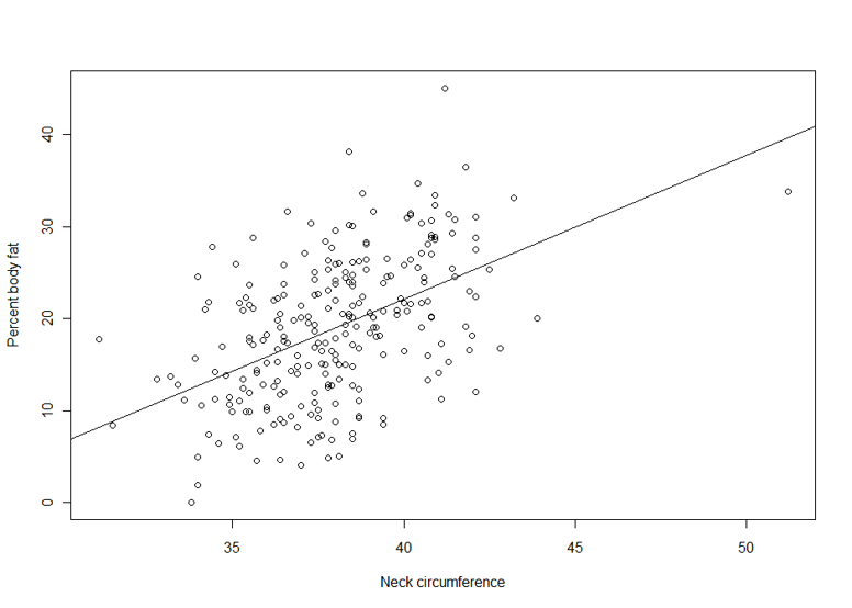Suppose we are interested in the relationship between body percent fat and neck circumference.

> lm1 <- lm(pctfat.brozek ~ neck, data = fatdata)

> plot(pctfat.brozek ~ neck, data = fatdata)

> abline(lm1)

> names(lm1)

[1] "coefficients" "residuals" "effects" "rank"

[5] "fitted.values" "assign" "qr" "df.residual"

[9] "xlevels" "call" "terms" "model"

> summary(lm1)

> lm1

Call:

lm(formula = pctfat.brozek ~ neck, data = fatdata)

Coefficients:

(Intercept) neck

-40.598 1.567

The argument pctfat.brozek ~ neck to lm function is a model formula. The resulting plot is shown in th figure on the right, and the abline() function extracts the coefficients of the fitted model and adds the corresponding regression line to the plot. The fitted-model object is stored as lm1, which is essentially a list.

The fitted model is pctfat.brozek = -40.598 + 1.567* neck. An lm object in fact contains more information than you just saw. For example, the basic extractor function is summary. The output from summary() is self-explanatory. For our model, we obtain

> summary(lm1)

Call:

lm(formula = pctfat.brozek ~ neck, data = fatdata) #This is the model formula

Residuals:

Min 1Q Median 3Q Max

-14.0076 -4.9450 -0.2405 5.0321 21.1344

Coefficients:

Estimate Std. Error t value Pr(>|t|) #These are the comprehensive results

(Intercept) -40.5985 6.6857 -6.072 4.66e-09 ***

neck 1.5671 0.1756 8.923 < 2e-16 ***

---

Signif. codes: 0 '***' 0.001 '**' 0.01 '*' 0.05 '.' 0.1 ' ' 1

Residual standard error: 6.764 on 250 degrees of freedom

Multiple R-squared: 0.2416, Adjusted R-squared: 0.2385

F-statistic: 79.62 on 1 and 250 DF, p-value: < 2.2e-16

The output provides a brief numerical summary of the residuals as well as a table of the estimated regression results.

Here the t-value of 8.923 and p-value of less than 2e-16 corresponds to the individual test of the hypothesis that "the true coefficient for variable neck equals 0". Also, two versions of r-squared tell us how much of the variation of the response variable is explained by our predictors, and not by error. In our case, the model explains around 24% of the variation of percent of body fat. The last row of results is the test for the hypothesis that all regression coefficients are zero.

When testing the null hypothesis that there is no linear association between neck size and Brozek percent fat we reject the null hypothesis (F_1,250 = 79.62, p-value < 2.2e-16, or t = 8.923, df = 250, p-value < 2.2e-16). For a one unit increase in neck there is a 1.57 increase in Brozek percent fat. Neck explains 24.16% of the variability in Brozek percent fat.

Fit a simple linear regression with pctfat.brozek as response variable and age as predictor.
What is the coefficient for variable age and how do you interpret this coefficient in the context?
Is age significantly associated with the percent of body fat? Provide evidence to support your argument.

Other Functions for Fitted Linear Model Objects

We have seen how summary can be used to extract information about the results of a regression analysis. In this session, we will introduce some more extraction functions. Table 4.2 lists generic function for fitted linear model objects. For example, we may obtain a plot of residuals versus fitted values via

> plot(fitted(lm1), resid(lm1))

> qqnorm(resid(lm1))

and check whether residuals might have come from a normal distribution by checking for a straight line on a Q-Q plot via qqnorm() function. The plot()function for class lm() provides six types of diagnostic plots, four of which are shown by default. Their discussion will be postponed until later. All plots may be accessed individually using the which argument, for example, plot(lm1, which=2), if only the QQ-plot is desired.

Generic functions for fitted (linear) model objects

Function	Description
print()	simple printed display
summary()	standard regression output
coef()	(or coefficients()) extracting the regression coefficients
residuals()	(or resid()) extracting residuals
fitted()	(or fitted.values()) extracting fitted values
anova()	comparison of nested models
predict()	predictions for new data
plot()	diagnostic plots
confint()	confidence intervals for the regression coefficients
deviance()	residual sum of squares
vcov()	(estimated) variance-covariance matrix
logLik()	log-likelihood (assuming normally distribted errors)
AIC	information criteria including AIC, BIC/SBC (assuming normally distributed errors)

Linear Regression in R (R Tutorial 5.1) MarinStatsLectures [Contents]

Multiple Linear Regression

Model Specification and Output

In reality, most regression analyses use more than a single predictor. Specification of a multiple regression analysis is done by setting up a model formula with plus (+) between the predictors:

> lm2<-lm(pctfat.brozek~age+fatfreeweight+neck,data=fatdata)

which corresponds to the following multiple linear regression model:

pctfat.brozek = β₀ + β₁*age + β₂*fatfreeweight + β₃*neck + ε

This tests the following hypotheses:

H₀: There is no linear association between pctfat.brozek and age, fatfreeweight and neck.
H_a: Here is a linear association between pctfat.brozek and age, fatfreeweight and neck.

> summary(lm2)

Call:

lm(formula = pctfat.brozek ~ age + fatfreeweight + neck, data = fatdata)

Residuals:

Min 1Q Median 3Q Max

-16.67871 -3.62536 0.07768 3.65100 16.99197

Coefficients:

Estimate Std. Error t value Pr(>|t|)

(Intercept) -53.01330 5.99614 -8.841 < 2e-16 ***

age 0.03832 0.03298 1.162 0.246

fatfreeweight -0.23200 0.03086 -7.518 1.02e-12 ***

neck 2.72617 0.22627 12.049 < 2e-16 ***

---

Signif. codes: 0 '***' 0.001 '**' 0.01 '*' 0.05 '.' 0.1 ' ' 1

Residual standard error: 5.901 on 248 degrees of freedom

Multiple R-squared: 0.4273, Adjusted R-squared: 0.4203

F-statistic: 61.67 on 3 and 248 DF, p-value: < 2.2e-16

Global Null Hypothesis

When testing the null hypothesis that there is no linear association between Brozek percent fat, age, fatfreeweight, and neck, we reject the null hypothesis (F_3,248 = 61.67, p-value < 2.2e-16). Age, fatfreeweight and neck explain 42.73% of the variability in Brozek percent fat.

Main Effects Hypothesis

When testing the null hypothesis that there is no linear association between Brozek percent fat and age after adjusting for fatfreeweight and neck, we fail to reject the null hypothesis (t = 1.162, df = 248, p-value = 0.246). For a one-unit change in age, on average, the Brozek percent fat increases by 0.03, after adjusting for fatfreeweight and neck.
When testing the null hypothesis that there is no linear association between Brozek percent fat and fatfreeweight after adjusting for age and neck, we reject the null hypothesis (t = -7.518, df = 248, p-value =1.02e-12). For a one-unit increase in fatfreeweight, Brozek percent fat decreases by 0.23 units after adjusting for age and neck.
When testing the null hypothesis that there is no linear association between Brozek percent fat and neck after adjusting for fatfreeweight and age, we reject the null hypothesis (t = 12.049, df = 248, p-value < 2e-16). For a one-unit increase in neck there is a 2.73 increase in Brozek percent fat, after adjusting for age and fatfreeweight.

Model with Categorical Variables or Factors

Sometimes, we may be also interested in using categorical variables as predictors. According to the information posted in the website of National Heart Lung and Blood Institute (http://www.nhlbi.nih.gov/health/public/heart/obesity/lose_wt/risk.htm), individuals with body mass index (BMI) greater than or equal to 25 are classified as overweight or obesity. In our dataset, the variable adiposity is equivalent to BMI.

Create a categorical variable bmi, which takes value of "overweight or obesity" if adiposity >= 25 and "normal or underweight" otherwise.

With the variable bmi you generated from the previous exercise, we go ahead to model our data.

> lm3 <- lm(pctfat.brozek ~ age + fatfreeweight + neck + factor(bmi), data = fatdata)

> summary(lm3)

Call:

lm(formula = pctfat.brozek ~ age + fatfreeweight + neck + factor(bmi),

data = fatdata)

Residuals:

Min 1Q Median 3Q Max

-13.4222 -3.0969 -0.2637 2.7280 13.3875

Coefficients:

Estimate Std. Error t value Pr(>|t|)

(Intercept) -21.31224 6.32852 -3.368 0.000879 ***

age 0.01698 0.02887 0.588 0.556890

fatfreeweight -0.23488 0.02691 -8.727 3.97e-16 ***

neck 1.83080 0.22152 8.265 8.63e-15 ***

factor(bmi)overweight or obesity 7.31761 0.82282 8.893 < 2e-16 ***

---

Signif. codes: 0 '***' 0.001 '**' 0.01 '*' 0.05 '.' 0.1 ' ' 1

Residual standard error: 5.146 on 247 degrees of freedom

Multiple R-squared: 0.5662, Adjusted R-squared: 0.5591

F-statistic: 80.59 on 4 and 247 DF, p-value: < 2.2e-16

Note that although factor bmi has two levels, the result only shows one level: "overweight or obesity", which is called the "treatment effect". In other words, the level "normal or underweight" is considered as baseline or reference group and the estimate of factor(bmi) overweight or obesity 7.3176 is the effect difference of these two levels on percent body fat.

Multiple Linear Regression in R (R Tutorial 5.3) MarinStatsLectures [Contents]

Regression Diagnostics

Model Assumptions

The model fitting is just the first part of the story for regression analysis since this is all based on certain assumptions. Regression diagnostics are used to evaluate the model assumptions and investigate whether or not there are observations with a large, undue influence on the analysis. Again, the assumptions for linear regression are:

Linearity: The relationship between X and the mean of Y is linear.
Homoscedasticity: The variance of residual is the same for any value of X.
Independence: Observations are independent of each other.
Normality: For any fixed value of X, Y is normally distributed.

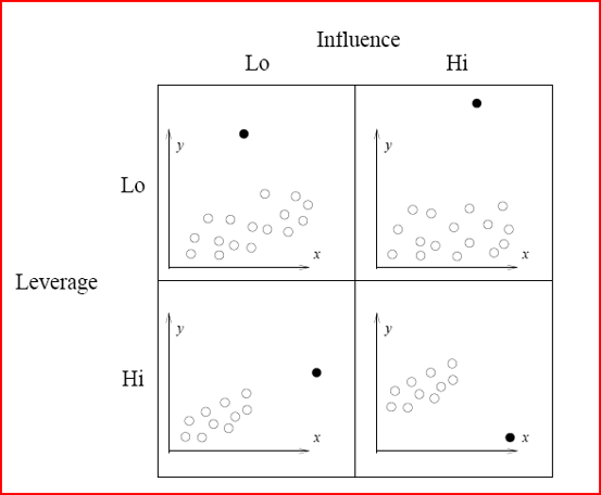
Before we go further, let's review some definitions for problematic points.

Outliers: an outlier is defined as an observation that has a large residual. In other words, the observed value for the point is very different from that predicted by the regression model.
Leverage points: A leverage point is defined as an observation that has a value of x that is far away from the mean of x.
Influential observations: An influential observation is defined as an observation that changes the slope of the line. Thus, influential points have a large influence on the fit of the model. One method to find influential points is to compare the fit of the model with and without each observation.

Illustration of Influence and leverage

Diagnostic Plots

The basic tool for examining the fit is the residuals. The plot() function provide 6 diagnostic plots and here we will introduce the first four. The plots are shown in Figure 2.

> par(mfrow=c(2,2))

> plot(lm3, which=1:4)

The first plot depicts residuals versus fitted values. Residuals are measured as follows:

residual = observed y – model-predicted y

The plot of residuals versus predicted values is useful for checking the assumption of linearity and homoscedasticity. If the model does not meet the linear model assumption, we would expect to see residuals that are very large (big positive value or big negative value). To assess the assumption of linearity we want to ensure that the residuals are not too far away from 0 (standardized values less than -2 or greater than 2 are deemed problematic). To assess if the homoscedasticity assumption is met we look to make sure that there is no pattern in the residuals and that they are equally spread around the y = 0 line.

The tests and intervals estimated in summary(lm3) are based on the assumption of normality. The normality assumption is evaluated based on the residuals and can be evaluated using a QQ-plot (plot 2) by comparing the residuals to "ideal" normal observations. Observations lie well along the 45-degree line in the QQ-plot, so we may assume that normality holds here.

The third plot is a scale-location plot (square rooted standardized residual vs. predicted value). This is useful for checking the assumption of homoscedasticity. In this particular plot we are checking to see if there is a pattern in the residuals.

The assumption of a random sample and independent observations cannot be tested with diagnostic plots. It is an assumption that you can test by examining the study design.

The fourth plot is of "Cook's distance", which is a measure of the influence of each observation on the regression coefficients. The Cook's distance statistic is a measure, for each observation in turn, of the extent of change in model estimates when that particular observation is omitted. Any observation for which the Cook's distance is close to 1 or more, or that is substantially larger than other Cook's distances (highly influential data points), requires investigation.

Outliers may or may not be influential points. Influential outliers are of the greatest concern. They should never be disregarded. Careful scrutiny of the original data may reveal an error in data entry that can be corrected. If they remain excluded from the final fitted model, they must be noted in the final report or paper.

Diagnostic Plots for Percent Body Fat Data

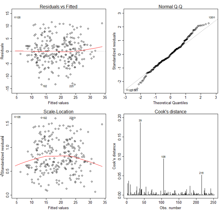
In our case, although observation 39 has larger Cook's distance than other data points in Cook's distance plot, this observation doesn't stand out in other plots. So we may decide to leave it in. A general rule-of-thumb is that a CD > k/n is noteworthy (k is # of predictors, n is sample size).

More Diagnostics

In addition to examining the diagnostic plots, it may be interesting and useful to examine, for each data point in turn, how removal of that point affects the regression coefficients, prediction and so on. To get these values, R has corresponding function to use: diffs(), dfbetas(), covratio(), hatvalues() and cooks.distance(). For example, we assess how many standard errors the predicted value changes when the ith observation is removed via the following command. (Note that here it doesn't show the result.)

> diffs(lm3)

Also, we can identify the leverage point via

> # list the observation with large hat value

> lm3.hat <- hatvalues(lm3)

> id.lm3.hat <- which(lm3.hat > (2*(4+1)/nrow(fatdata))) ## hatvalue > #2*(k+1)/n

> lm3.hat[id.lm3.hat]

5 9 12 28 39 79 106

0.04724447 0.04100957 0.05727609 0.06020518 0.17631101 0.04596512 0.06125064

207 216 235

0.04501627 0.05087598 0.05863139

It indicates potential influential observations for 10 data points. This tells us that we need to pay attention to observations 5, 9, 12, 28, 39, 79, 106, 207, 216 and 235. If we also see these points standing out in other diagnostics, then more investigation might be warned.

Information for influence.measures() function. K = # (predictor)

Function	Description	Rough Cut-off
dffits()	the change in the fitted values (with appropriately scaled)	> 2*sqrt{(k+1)/n}
dfbetas()	the changes in the coefficients (with appropriately scaled)	> 2/sqrt(n)
covratio()	the change in the estimate of OLS covariance matrix	outside 1+/- 3*(k+1)/n
hatvalues()	standardized distance to mean of predictors used to measure the leverage of observation	> 2*(k+1)/n
cooks.distance()	standardized distance change for how far the estimate vector	> 4/n

Fortunately, it is not necessary to compute all the preceding quantities separately (although it is possible). R provides the convenience function influence.measures(), which simultaneously calls these functions (listed in Table 4.3). Note that the cut-off listed in Table 3 is just a suggestive point. It doesn't mean we always need to delete the points which are outside of cut-off points.

> summary(influence.measures(lm3))

Potentially influential observations of

lm(formula = pctfat.brozek ~ age + fatfreeweight + neck + factor(bmi), data = fatdata) :

dfb.1_ dfb.age dfb.ftfr dfb.neck dfb.f(oo dffit cov.r cook.d hat

5 0.35 -0.20 -0.01 -0.24 0.32 0.43_* 0.99 0.04 0.05

9 0.00 0.01 -0.04 0.01 0.02 -0.05 1.06_* 0.00 0.04

12 -0.04 0.00 -0.15 0.10 -0.04 -0.18 1.07_* 0.01 0.06

28 0.02 0.03 0.04 -0.03 0.02 -0.04 1.09_* 0.00 0.06_*

39 -0.81 0.10 0.33 0.47 -0.43 0.97_* 1.13_* 0.19 0.18_*

55 0.12 0.10 0.20 -0.21 0.20 -0.33 0.90_* 0.02 0.02

79 -0.02 0.06 0.00 0.01 -0.03 0.07 1.07_* 0.00 0.05

98 -0.05 -0.03 0.02 0.03 -0.16 -0.24 0.90_* 0.01 0.01

106 0.57 0.19 0.41 -0.65 0.16 0.69_* 0.94_* 0.09 0.06_*

138 -0.09 -0.05 -0.10 0.13 -0.17 0.25 0.93_* 0.01 0.01

182 -0.24 0.06 0.07 0.13 -0.01 -0.35 0.90_* 0.02 0.02

207 0.00 0.00 0.00 0.00 0.00 0.00 1.07_* 0.00 0.05

216 -0.21 -0.15 -0.45 0.39 0.03 0.51_* 0.97 0.05 0.05

225 0.15 -0.12 -0.05 -0.07 -0.03 -0.30 0.90_* 0.02 0.01

235 0.02 0.00 0.02 -0.02 0.02 -0.03 1.08_* 0.00 0.06

There is a lot I am not covering here. There is a vast literature around choosing the best model (covariates), how to proceed when assumptions are violated, and what to do about collinearity among the predictors (Ridge Regression/LASSO). If anyone is interested we could have a brief overview of a fun topic for dealing with multicollinearity: Ridge Regression.

Checking Linear Regression Assumptions in R (R Tutorial 5.2) MarinStatsLectures [Contents]

Reading:

VS Chapter 11.1-11.3
R Manual for BS 704: Sections 4.1, 4.2

Assignment:

Homework 4 and final project proposal due, Homework 4 assigned.

Reference

Penrose, K., Nelson, A., and Fisher, A. (1985), "Generalized Body Composition Prediction Equation for Men Using Simple Measurement Techniques" (abstract), Medicine and Science in Sports and Exercise, 17(2), 189.