

Regression Diagnostics
Model Assumptions
The model fitting is just the first part of the story for regression analysis since this is all based on certain assumptions. Regression diagnostics are used to evaluate the model assumptions and investigate whether or not there are observations with a large, undue influence on the analysis. Again, the assumptions for linear regression are:
- Linearity: The relationship between X and the mean of Y is linear.
- Homoscedasticity: The variance of residual is the same for any value of X.
- Independence: Observations are independent of each other.
- Normality: For any fixed value of X, Y is normally distributed.
Before we go further, let's review some definitions for problematic points.
- Outliers: an outlier is defined as an observation that has a large residual. In other words, the observed value for the point is very different from that predicted by the regression model.
- Leverage points: A leverage point is defined as an observation that has a value of x that is far away from the mean of x.
- Influential observations: An influential observation is defined as an observation that changes the slope of the line. Thus, influential points have a large influence on the fit of the model. One method to find influential points is to compare the fit of the model with and without each observation.
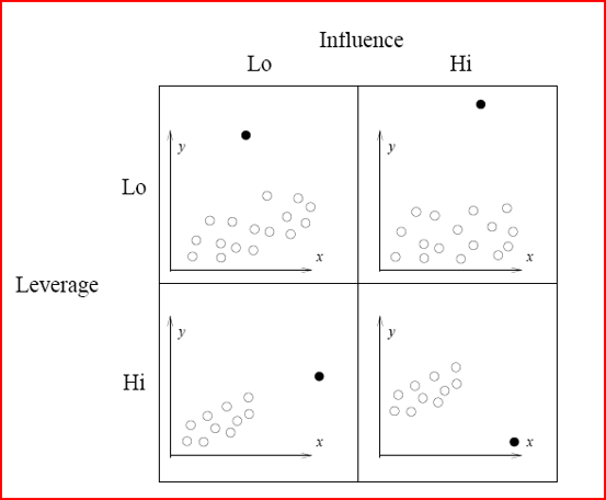
Illustration of Influence and leverage
Diagnostic Plots
The basic tool for examining the fit is the residuals. The plot() function provide 6 diagnostic plots and here we will introduce the first four. The plots are shown in Figure 2.
> par(mfrow=c(2,2))
> plot(lm3, which=1:4)
The first plot depicts residuals versus fitted values. Residuals are measured as follows:
residual = observed y – model-predicted y
The plot of residuals versus predicted values is useful for checking the assumption of linearity and homoscedasticity. If the model does not meet the linear model assumption, we would expect to see residuals that are very large (big positive value or big negative value). To assess the assumption of linearity we want to ensure that the residuals are not too far away from 0 (standardized values less than -2 or greater than 2 are deemed problematic). To assess if the homoscedasticity assumption is met we look to make sure that there is no pattern in the residuals and that they are equally spread around the y = 0 line.
The tests and intervals estimated in summary(lm3) are based on the assumption of normality. The normality assumption is evaluated based on the residuals and can be evaluated using a QQ-plot (plot 2) by comparing the residuals to "ideal" normal observations. Observations lie well along the 45-degree line in the QQ-plot, so we may assume that normality holds here.
The third plot is a scale-location plot (square rooted standardized residual vs. predicted value). This is useful for checking the assumption of homoscedasticity. In this particular plot we are checking to see if there is a pattern in the residuals.
The assumption of a random sample and independent observations cannot be tested with diagnostic plots. It is an assumption that you can test by examining the study design.
The fourth plot is of "Cook's distance", which is a measure of the influence of each observation on the regression coefficients. The Cook's distance statistic is a measure, for each observation in turn, of the extent of change in model estimates when that particular observation is omitted. Any observation for which the Cook's distance is close to 1 or more, or that is substantially larger than other Cook's distances (highly influential data points), requires investigation.
Outliers may or may not be influential points. Influential outliers are of the greatest concern. They should never be disregarded. Careful scrutiny of the original data may reveal an error in data entry that can be corrected. If they remain excluded from the final fitted model, they must be noted in the final report or paper.
Diagnostic Plots for Percent Body Fat Data
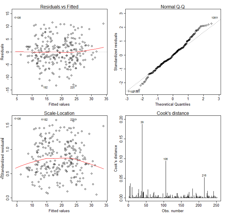
In our case, although observation 39 has larger Cook's distance than other data points in Cook's distance plot, this observation doesn't stand out in other plots. So we may decide to leave it in. A general rule-of-thumb is that a CD > k/n is noteworthy (k is # of predictors, n is sample size).
More Diagnostics
In addition to examining the diagnostic plots, it may be interesting and useful to examine, for each data point in turn, how removal of that point affects the regression coefficients, prediction and so on. To get these values, R has corresponding function to use: diffs(), dfbetas(), covratio(), hatvalues() and cooks.distance(). For example, we assess how many standard errors the predicted value changes when the ith observation is removed via the following command. (Note that here it doesn't show the result.)
> diffs(lm3)
Also, we can identify the leverage point via
> # list the observation with large hat value
> lm3.hat <- hatvalues(lm3)
> id.lm3.hat <- which(lm3.hat > (2*(4+1)/nrow(fatdata))) ## hatvalue > #2*(k+1)/n
> lm3.hat[id.lm3.hat]
5 9 12 28 39 79 106
0.04724447 0.04100957 0.05727609 0.06020518 0.17631101 0.04596512 0.06125064
207 216 235
0.04501627 0.05087598 0.05863139
>
It indicates potential influential observations for 10 data points. This tells us that we need to pay attention to observations 5, 9, 12, 28, 39, 79, 106, 207, 216 and 235. If we also see these points standing out in other diagnostics, then more investigation might be warned.
Information for influence.measures() function. K = # (predictor)
| Function |
Description |
Rough Cut-off |
|---|---|---|
|
dffits() |
the change in the fitted values (with appropriately scaled) |
> 2*sqrt{(k+1)/n} |
|
dfbetas() |
the changes in the coefficients (with appropriately scaled) |
> 2/sqrt(n) |
|
covratio() |
the change in the estimate of OLS covariance matrix |
outside 1+/- 3*(k+1)/n |
|
hatvalues() |
standardized distance to mean of predictors used to measure the leverage of observation |
> 2*(k+1)/n |
|
cooks.distance() |
standardized distance change for how far the estimate vector |
> 4/n |
Fortunately, it is not necessary to compute all the preceding quantities separately (although it is possible). R provides the convenience function influence.measures(), which simultaneously calls these functions (listed in Table 4.3). Note that the cut-off listed in Table 3 is just a suggestive point. It doesn't mean we always need to delete the points which are outside of cut-off points.
> summary(influence.measures(lm3))
Potentially influential observations of
lm(formula = pctfat.brozek ~ age + fatfreeweight + neck + factor(bmi), data = fatdata) :
dfb.1_ dfb.age dfb.ftfr dfb.neck dfb.f(oo dffit cov.r cook.d hat
5 0.35 -0.20 -0.01 -0.24 0.32 0.43_* 0.99 0.04 0.05
9 0.00 0.01 -0.04 0.01 0.02 -0.05 1.06_* 0.00 0.04
12 -0.04 0.00 -0.15 0.10 -0.04 -0.18 1.07_* 0.01 0.06
28 0.02 0.03 0.04 -0.03 0.02 -0.04 1.09_* 0.00 0.06_*
39 -0.81 0.10 0.33 0.47 -0.43 0.97_* 1.13_* 0.19 0.18_*
55 0.12 0.10 0.20 -0.21 0.20 -0.33 0.90_* 0.02 0.02
79 -0.02 0.06 0.00 0.01 -0.03 0.07 1.07_* 0.00 0.05
98 -0.05 -0.03 0.02 0.03 -0.16 -0.24 0.90_* 0.01 0.01
106 0.57 0.19 0.41 -0.65 0.16 0.69_* 0.94_* 0.09 0.06_*
138 -0.09 -0.05 -0.10 0.13 -0.17 0.25 0.93_* 0.01 0.01
182 -0.24 0.06 0.07 0.13 -0.01 -0.35 0.90_* 0.02 0.02
207 0.00 0.00 0.00 0.00 0.00 0.00 1.07_* 0.00 0.05
216 -0.21 -0.15 -0.45 0.39 0.03 0.51_* 0.97 0.05 0.05
225 0.15 -0.12 -0.05 -0.07 -0.03 -0.30 0.90_* 0.02 0.01
235 0.02 0.00 0.02 -0.02 0.02 -0.03 1.08_* 0.00 0.06
>
There is a lot I am not covering here. There is a vast literature around choosing the best model (covariates), how to proceed when assumptions are violated, and what to do about collinearity among the predictors (Ridge Regression/LASSO). If anyone is interested we could have a brief overview of a fun topic for dealing with multicollinearity: Ridge Regression.
Checking Linear Regression Assumptions in R (R Tutorial 5.2) MarinStatsLectures [Contents ]
]
![]()
![]()
Reading:
- VS Chapter 11.1-11.3
- R Manual for BS 704: Sections 4.1, 4.2
Assignment:
- Homework 4 and final project proposal due, Homework 4 assigned.
Reference
- Penrose, K., Nelson, A., and Fisher, A. (1985), "Generalized Body Composition Prediction Equation for Men Using Simple Measurement Techniques" (abstract), Medicine and Science in Sports and Exercise, 17(2), 189.
