


Simple Linear Regression Model Fitting
The fat data frame contains 252 observations (individuals) on 19 variables. Here we don't need all the variables, so let's create a smaller dataset to use.
> fatdata<-fat[,c(1,2,5:11)]
> summary(fatdata[,-1]) # do you remember what the negative index (-1) here means?
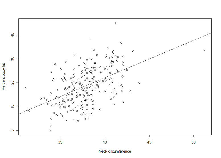 Suppose we are interested in the relationship between body percent fat and neck circumference.
> lm1 <- lm(pctfat.brozek ~ neck, data = fatdata)
> plot(pctfat.brozek ~ neck, data = fatdata)
> abline(lm1)
> names(lm1)
[1] "coefficients" "residuals" "effects" "rank"
[5] "fitted.values" "assign" "qr" "df.residual"
[9] "xlevels" "call" "terms" "model"
> summary(lm1)
> lm1
Call:
lm(formula = pctfat.brozek ~ neck, data = fatdata)
Coefficients:
(Intercept) neck
-40.598 1.567
The argument pctfat.brozek ~ neck to lm function is a model formula. The resulting plot is shown in th figure on the right, and the abline() function extracts the coefficients of the fitted model and adds the corresponding regression line to the plot. The fitted-model object is stored as lm1, which is essentially a list.
The fitted model is pctfat.brozek = -40.598 + 1.567* neck. An lm object in fact contains more information than you just saw. For example, the basic extractor function is summary. The output from summary() is self-explanatory. For our model, we obtain
> summary(lm1)
Call:
lm(formula = pctfat.brozek ~ neck, data = fatdata) #This is the model formula
Residuals:
Min 1Q Median 3Q Max
-14.0076 -4.9450 -0.2405 5.0321 21.1344
Coefficients:
Estimate Std. Error t value Pr(>|t|) #These are the comprehensive results
(Intercept) -40.5985 6.6857 -6.072 4.66e-09 ***
neck 1.5671 0.1756 8.923 < 2e-16 ***
---
Signif. codes: 0 '***' 0.001 '**' 0.01 '*' 0.05 '.' 0.1 ' ' 1
Residual standard error: 6.764 on 250 degrees of freedom
Multiple R-squared: 0.2416, Adjusted R-squared: 0.2385
F-statistic: 79.62 on 1 and 250 DF, p-value: < 2.2e-16
The output provides a brief numerical summary of the residuals as well as a table of the estimated regression results.
Here the t-value of 8.923 and p-value of less than 2e-16 corresponds to the individual test of the hypothesis that "the true coefficient for variable neck equals 0". Also, two versions of r-squared tell us how much of the variation of the response variable is explained by our predictors, and not by error. In our case, the model explains around 24% of the variation of percent of body fat. The last row of results is the test for the hypothesis that all regression coefficients are zero.
When testing the null hypothesis that there is no linear association between neck size and Brozek percent fat we reject the null hypothesis (F1,250 = 79.62, p-value < 2.2e-16, or t = 8.923, df = 250, p-value < 2.2e-16). For a one unit increase in neck there is a 1.57 increase in Brozek percent fat. Neck explains 24.16% of the variability in Brozek percent fat.
|
|

Other Functions for Fitted Linear Model Objects
We have seen how summary can be used to extract information about the results of a regression analysis. In this session, we will introduce some more extraction functions. Table 4.2 lists generic function for fitted linear model objects. For example, we may obtain a plot of residuals versus fitted values via
> plot(fitted(lm1), resid(lm1))
> qqnorm(resid(lm1))
and check whether residuals might have come from a normal distribution by checking for a straight line on a Q-Q plot via qqnorm() function. The plot()function for class lm() provides six types of diagnostic plots, four of which are shown by default. Their discussion will be postponed until later. All plots may be accessed individually using the which argument, for example, plot(lm1, which=2), if only the QQ-plot is desired.
Generic functions for fitted (linear) model objects
| Function |
Description |
|---|---|
|
print() |
simple printed display |
|
summary() |
standard regression output |
|
coef() |
(or coefficients()) extracting the regression coefficients |
|
residuals() |
(or resid()) extracting residuals |
|
fitted() |
(or fitted.values()) extracting fitted values |
|
anova() |
comparison of nested models |
|
predict() |
predictions for new data |
|
plot() |
diagnostic plots |
|
confint() |
confidence intervals for the regression coefficients |
|
deviance() |
residual sum of squares |
|
vcov() |
(estimated) variance-covariance matrix |
|
logLik() |
log-likelihood (assuming normally distribted errors) |
|
AIC |
information criteria including AIC, BIC/SBC (assuming normally distributed errors) |
Linear Regression in R (R Tutorial 5.1) MarinStatsLectures [Contents ]
]
![]()
![]()
