


Sample Sizes for Two Independent Samples, Continuous Outcome
In studies where the plan is to estimate the difference in means between two independent populations, the formula for determining the sample sizes required in each comparison group is given below:


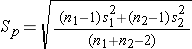
where ni is the sample size required in each group (i=1,2), Z is the value from the standard normal distribution reflecting the confidence level that will be used and E is the desired margin of error. σ again reflects the standard deviation of the outcome variable. Recall from the module on confidence intervals that, when we generated a confidence interval estimate for the difference in means, we used Sp, the pooled estimate of the common standard deviation, as a measure of variability in the outcome (based on pooling the data), where Sp is computed as follows:
If data are available on variability of the outcome in each comparison group, then Sp can be computed and used in the sample size formula. However, it is more often the case that data on the variability of the outcome are available from only one group, often the untreated (e.g., placebo control) or unexposed group. When planning a clinical trial to investigate a new drug or procedure, data are often available from other trials that involved a placebo or an active control group (i.e., a standard medication or treatment given for the condition under study). The standard deviation of the outcome variable measured in patients assigned to the placebo, control or unexposed group can be used to plan a future trial, as illustrated below.
Note that the formula for the sample size generates sample size estimates for samples of equal size. If a study is planned where different numbers of patients will be assigned or different numbers of patients will comprise the comparison groups, then alternative formulas can be used.
Example 4:
An investigator wants to plan a clinical trial to evaluate the efficacy of a new drug designed to increase HDL cholesterol (the "good" cholesterol). The plan is to enroll participants and to randomly assign them to receive either the new drug or a placebo. HDL cholesterol will be measured in each participant after 12 weeks on the assigned treatment. Based on prior experience with similar trials, the investigator expects that 10% of all participants will be lost to follow up or will drop out of the study over 12 weeks. A 95% confidence interval will be estimated to quantify the difference in mean HDL levels between patients taking the new drug as compared to placebo. The investigator would like the margin of error to be no more than 3 units. How many patients should be recruited into the study?
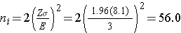
The sample sizes are computed as follows:
A major issue is determining the variability in the outcome of interest (σ), here the standard deviation of HDL cholesterol. To plan this study, we can use data from the Framingham Heart Study. In participants who attended the seventh examination of the Offspring Study and were not on treatment for high cholesterol, the standard deviation of HDL cholesterol is 17.1. We will use this value and the other inputs to compute the sample sizes as follows:
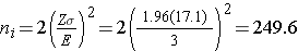
Samples of size n1=250 and n2=250 will ensure that the 95% confidence interval for the difference in mean HDL levels will have a margin of error of no more than 3 units. Again, these sample sizes refer to the numbers of participants with complete data. The investigators hypothesized a 10% attrition (or drop-out) rate (in both groups). In order to ensure that the total sample size of 500 is available at 12 weeks, the investigator needs to recruit more participants to allow for attrition.
N (number to enroll) * (% retained) = desired sample size
Therefore N (number to enroll) = desired sample size/(% retained)
N = 500/0.90 = 556
If they anticipate a 10% attrition rate, the investigators should enroll 556 participants. This will ensure N=500 with complete data at the end of the trial.
Example 5:
An investigator wants to compare two diet programs in children who are obese. One diet is a low fat diet, and the other is a low carbohydrate diet. The plan is to enroll children and weigh them at the start of the study. Each child will then be randomly assigned to either the low fat or the low carbohydrate diet. Each child will follow the assigned diet for 8 weeks, at which time they will again be weighed. The number of pounds lost will be computed for each child. Based on data reported from diet trials in adults, the investigator expects that 20% of all children will not complete the study. A 95% confidence interval will be estimated to quantify the difference in weight lost between the two diets and the investigator would like the margin of error to be no more than 3 pounds. How many children should be recruited into the study?
The sample sizes are computed as follows:
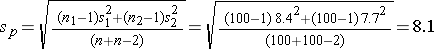
Again the issue is determining the variability in the outcome of interest (σ), here the standard deviation in pounds lost over 8 weeks. To plan this study, investigators use data from a published study in adults. Suppose one such study compared the same diets in adults and involved 100 participants in each diet group. The study reported a standard deviation in weight lost over 8 weeks on a low fat diet of 8.4 pounds and a standard deviation in weight lost over 8 weeks on a low carbohydrate diet of 7.7 pounds. These data can be used to estimate the common standard deviation in weight lost as follows:
We now use this value and the other inputs to compute the sample sizes:
Samples of size n1=56 and n2=56 will ensure that the 95% confidence interval for the difference in weight lost between diets will have a margin of error of no more than 3 pounds. Again, these sample sizes refer to the numbers of children with complete data. The investigators anticipate a 20% attrition rate. In order to ensure that the total sample size of 112 is available at 8 weeks, the investigator needs to recruit more participants to allow for attrition.
N (number to enroll) * (% retained) = desired sample size
Therefore N (number to enroll) = desired sample size/(% retained)
N = 112/0.80 = 140
Sample Size for Matched Samples, Continuous Outcome
In studies where the plan is to estimate the mean difference of a continuous outcome based on matched data, the formula for determining sample size is given below:

where Z is the value from the standard normal distribution reflecting the confidence level that will be used (e.g., Z = 1.96 for 95%), E is the desired margin of error, and σd is the standard deviation of the difference scores. It is extremely important that the standard deviation of the difference scores (e.g., the difference based on measurements over time or the difference between matched pairs) is used here to appropriately estimate the sample size.
Sample Sizes for Two Independent Samples, Dichotomous Outcome
In studies where the plan is to estimate the difference in proportions between two independent populations (i.e., to estimate the risk difference), the formula for determining the sample sizes required in each comparison group is:
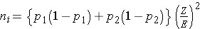
where ni is the sample size required in each group (i=1,2), Z is the value from the standard normal distribution reflecting the confidence level that will be used (e.g., Z = 1.96 for 95%), and E is the desired margin of error. p1 and p2 are the proportions of successes in each comparison group. Again, here we are planning a study to generate a 95% confidence interval for the difference in unknown proportions, and the formula to estimate the sample sizes needed requires p1 and p2. In order to estimate the sample size, we need approximate values of p1 and p2. The values of p1 and p2 that maximize the sample size are p1=p2=0.5. Thus, if there is no information available to approximate p1 and p2, then 0.5 can be used to generate the most conservative, or largest, sample sizes.
Similar to the situation for two independent samples and a continuous outcome at the top of this page, it may be the case that data are available on the proportion of successes in one group, usually the untreated (e.g., placebo control) or unexposed group. If so, the known proportion can be used for both p1 and p2 in the formula shown above. The formula shown above generates sample size estimates for samples of equal size. If a study is planned where different numbers of patients will be assigned or different numbers of patients will comprise the comparison groups, then alternative formulas can be used. Interested readers can see Fleiss for more details.4
Example 6:
An investigator wants to estimate the impact of smoking during pregnancy on premature delivery. Normal pregnancies last approximately 40 weeks and premature deliveries are those that occur before 37 weeks. The 2005 National Vital Statistics report indicates that approximately 12% of infants are born prematurely in the United States.5 The investigator plans to collect data through medical record review and to generate a 95% confidence interval for the difference in proportions of infants born prematurely to women who smoked during pregnancy as compared to those who did not. How many women should be enrolled in the study to ensure that the 95% confidence interval for the difference in proportions has a margin of error of no more than 4%?
The sample sizes (i.e., numbers of women who smoked and did not smoke during pregnancy) can be computed using the formula shown above. National data suggest that 12% of infants are born prematurely. We will use that estimate for both groups in the sample size computation.

Samples of size n1=508 women who smoked during pregnancy and n2=508 women who did not smoke during pregnancy will ensure that the 95% confidence interval for the difference in proportions who deliver prematurely will have a margin of error of no more than 4%.

Is attrition an issue here?