Hypothesis Testing - Analysis of Variance (ANOVA)
Author:
Lisa Sullivan, PhD
Professor of Biostatistics
Boston University School of Public Health
This module will continue the discussion of hypothesis testing, where a specific statement or hypothesis is generated about a population parameter, and sample statistics are used to assess the likelihood that the hypothesis is true. The hypothesis is based on available information and the investigator's belief about the population parameters. The specific test considered here is called analysis of variance (ANOVA) and is a test of hypothesis that is appropriate to compare means of a continuous variable in two or more independent comparison groups. For example, in some clinical trials there are more than two comparison groups. In a clinical trial to evaluate a new medication for asthma, investigators might compare an experimental medication to a placebo and to a standard treatment (i.e., a medication currently being used). In an observational study such as the Framingham Heart Study, it might be of interest to compare mean blood pressure or mean cholesterol levels in persons who are underweight, normal weight, overweight and obese.
The technique to test for a difference in more than two independent means is an extension of the two independent samples procedure discussed previously which applies when there are exactly two independent comparison groups. The ANOVA technique applies when there are two or more than two independent groups. The ANOVA procedure is used to compare the means of the comparison groups and is conducted using the same five step approach used in the scenarios discussed in previous sections. Because there are more than two groups, however, the computation of the test statistic is more involved. The test statistic must take into account the sample sizes, sample means and sample standard deviations in each of the comparison groups.
If one is examining the means observed among, say three groups, it might be tempting to perform three separate group to group comparisons, but this approach is incorrect because each of these comparisons fails to take into account the total data, and it increases the likelihood of incorrectly concluding that there are statistically significate differences, since each comparison adds to the probability of a type I error. Analysis of variance avoids these problemss by asking a more global question, i.e., whether there are significant differences among the groups, without addressing differences between any two groups in particular (although there are additional tests that can do this if the analysis of variance indicates that there are differences among the groups).
The fundamental strategy of ANOVA is to systematically examine variability within groups being compared and also examine variability among the groups being compared.
After completing this module, the student will be able to:

Consider an example with four independent groups and a continuous outcome measure. The independent groups might be defined by a particular characteristic of the participants such as BMI (e.g., underweight, normal weight, overweight, obese) or by the investigator (e.g., randomizing participants to one of four competing treatments, call them A, B, C and D). Suppose that the outcome is systolic blood pressure, and we wish to test whether there is a statistically significant difference in mean systolic blood pressures among the four groups. The sample data are organized as follows:
|
|
Group 1 |
Group 2 |
Group 3 |
Group 4 |
|---|---|---|---|---|
|
Sample Size |
n1 |
n2 |
n3 |
n4 |
|
Sample Mean |
|
|
|
|
|
Sample Standard Deviation |
s1 |
s2 |
s3 |
s4 |
The hypotheses of interest in an ANOVA are as follows:
where k = the number of independent comparison groups.
In this example, the hypotheses are:
The null hypothesis in ANOVA is always that there is no difference in means. The research or alternative hypothesis is always that the means are not all equal and is usually written in words rather than in mathematical symbols. The research hypothesis captures any difference in means and includes, for example, the situation where all four means are unequal, where one is different from the other three, where two are different, and so on. The alternative hypothesis, as shown above, capture all possible situations other than equality of all means specified in the null hypothesis.
The test statistic for testing H0: μ1 = μ2 = ... = μk is:
and the critical value is found in a table of probability values for the F distribution with (degrees of freedom) df1 = k-1, df2=N-k. The table can be found in "Other Resources" on the left side of the pages.
In the test statistic, nj = the sample size in the jth group (e.g., j =1, 2, 3, and 4 when there are 4 comparison groups),  is the sample mean in the jth group, and
  is the overall mean. k represents the number of independent groups (in this example, k=4), and N represents the total number of observations in the analysis. Note that N does not refer to a population size, but instead to the total sample size in the analysis (the sum of the sample sizes in the comparison groups, e.g., N=n1+n2+n3+n4). The test statistic is complicated because it incorporates all of the sample data. While it is not easy to see the extension, the F statistic shown above is a generalization of the test statistic used for testing the equality of exactly two means.
NOTE: The test statistic F assumes equal variability in the k populations (i.e., the population variances are equal, or s12 = s22 = ... = sk2 ). This means that the outcome is equally variable in each of the comparison populations. This assumption is the same as that assumed for appropriate use of the test statistic to test equality of two independent means. It is possible to assess the likelihood that the assumption of equal variances is true and the test can be conducted in most statistical computing packages. If the variability in the k comparison groups is not similar, then alternative techniques must be used.
The F statistic is computed by taking the ratio of what is called the "between treatment" variability to the "residual or error" variability. This is where the name of the procedure originates. In analysis of variance we are testing for a difference in means (H0: means are all equal versus H1: means are not all equal) by evaluating variability in the data. The numerator captures between treatment variability (i.e., differences among the sample means) and the denominator contains an estimate of the variability in the outcome. The test statistic is a measure that allows us to assess whether the differences among the sample means (numerator) are more than would be expected by chance if the null hypothesis is true. Recall in the two independent sample test, the test statistic was computed by taking the ratio of the difference in sample means (numerator) to the variability in the outcome (estimated by Sp).
The decision rule for the F test in ANOVA is set up in a similar way to decision rules we established for t tests. The decision rule again depends on the level of significance and the degrees of freedom. The F statistic has two degrees of freedom. These are denoted df1 and df2, and called the numerator and denominator degrees of freedom, respectively. The degrees of freedom are defined as follows:
df1 = k-1 and df2=N-k,
where k is the number of comparison groups and N is the total number of observations in the analysis. If the null hypothesis is true, the between treatment variation (numerator) will not exceed the residual or error variation (denominator) and the F statistic will small. If the null hypothesis is false, then the F statistic will be large. The rejection region for the F test is always in the upper (right-hand) tail of the distribution as shown below.
Rejection Region for F Test with a =0.05, df1=3 and df2=36 (k=4, N=40)
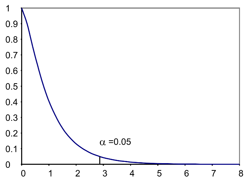
For the scenario depicted here, the decision rule is: Reject H0 if F > 2.87.
We will next illustrate the ANOVA procedure using the five step approach. Because the computation of the test statistic is involved, the computations are often organized in an ANOVA table. The ANOVA table breaks down the components of variation in the data into variation between treatments and error or residual variation. Statistical computing packages also produce ANOVA tables as part of their standard output for ANOVA, and the ANOVA table is set up as follows:
|
Source of Variation |
Sums of Squares (SS) |
Degrees of Freedom (df) |
Mean Squares (MS) |
F |
|---|---|---|---|---|
|
Between Treatments |
|
k-1 |
|
|
|
Error (or Residual) |
|
N-k |
|
|
|
Total |
|
N-1 |
where
 = sample mean of the jth treatment (or group),
 = overall sample mean,
The ANOVA table above is organized as follows.
and is computed by summing the squared differences between each treatment (or group) mean and the overall mean. The squared differences are weighted by the sample sizes per group (nj). The error sums of squares is:
and is computed by summing the squared differences between each observation and its group mean (i.e., the squared differences between each observation in group 1 and the group 1 mean, the squared differences between each observation in group 2 and the group 2 mean, and so on). The double summation ( SS ) indicates summation of the squared differences within each treatment and then summation of these totals across treatments to produce a single value. (This will be illustrated in the following examples). The total sums of squares is:
and is computed by summing the squared differences between each observation and the overall sample mean. In an ANOVA, data are organized by comparison or treatment groups. If all of the data were pooled into a single sample, SST would reflect the numerator of the sample variance computed on the pooled or total sample. SST does not figure into the F statistic directly. However, SST = SSB + SSE, thus if two sums of squares are known, the third can be computed from the other two.
Example:
A clinical trial is run to compare weight loss programs and participants are randomly assigned to one of the comparison programs and are counseled on the details of the assigned program. Participants follow the assigned program for 8 weeks. The outcome of interest is weight loss, defined as the difference in weight measured at the start of the study (baseline) and weight measured at the end of the study (8 weeks), measured in pounds.
Three popular weight loss programs are considered. The first is a low calorie diet. The second is a low fat diet and the third is a low carbohydrate diet. For comparison purposes, a fourth group is considered as a control group. Participants in the fourth group are told that they are participating in a study of healthy behaviors with weight loss only one component of interest. The control group is included here to assess the placebo effect (i.e., weight loss due to simply participating in the study). A total of twenty patients agree to participate in the study and are randomly assigned to one of the four diet groups. Weights are measured at baseline and patients are counseled on the proper implementation of the assigned diet (with the exception of the control group). After 8 weeks, each patient's weight is again measured and the difference in weights is computed by subtracting the 8 week weight from the baseline weight. Positive differences indicate weight losses and negative differences indicate weight gains. For interpretation purposes, we refer to the differences in weights as weight losses and the observed weight losses are shown below.
|
Low Calorie |
Low Fat |
Low Carbohydrate |
Control |
|---|---|---|---|
|
8 |
2 |
3 |
2 |
|
9 |
4 |
5 |
2 |
|
6 |
3 |
4 |
-1 |
|
7 |
5 |
2 |
0 |
|
3 |
1 |
3 |
3 |
Is there a statistically significant difference in the mean weight loss among the four diets? We will run the ANOVA using the five-step approach.
H0: μ1 = μ2 = μ3 = μ4 H1: Means are not all equal α=0.05
The test statistic is the F statistic for ANOVA, F=MSB/MSE.
The appropriate critical value can be found in a table of probabilities for the F distribution(see "Other Resources"). In order to determine the critical value of F we need degrees of freedom, df1=k-1 and df2=N-k. In this example, df1=k-1=4-1=3 and df2=N-k=20-4=16. The critical value is 3.24 and the decision rule is as follows: Reject H0 if F > 3.24.
To organize our computations we complete the ANOVA table. In order to compute the sums of squares we must first compute the sample means for each group and the overall mean based on the total sample.
|
|
Low Calorie |
Low Fat |
Low Carbohydrate |
Control |
|---|---|---|---|---|
|
n |
5 |
5 |
5 |
5 |
|
Group mean |
6.6 |
3.0 |
3.4 |
1.2 |
If we pool all N=20 observations, the overall mean is  = 3.6.
We can now compute
So, in this case:


Next we compute,
SSE requires computing the squared differences between each observation and its group mean. We will compute SSE in parts. For the participants in the low calorie diet:
|
Low Calorie |
(X - 6.6) |
(X - 6.6)2 |
|---|---|---|
|
8 |
1.4 |
2.0 |
|
9 |
2.4 |
5.8 |
|
6 |
-0.6 |
0.4 |
|
7 |
0.4 |
0.2 |
|
3 |
-3.6 |
13.0 |
| Totals |
0 |
21.4 |
Thus, 
For the participants in the low fat diet:
|
Low Fat |
(X - 3.0) |
(X - 3.0)2 |
|---|---|---|
|
2 |
-1.0 |
1.0 |
|
4 |
1.0 |
1.0 |
|
3 |
0.0 |
0.0 |
|
5 |
2.0 |
4.0 |
|
1 |
-2.0 |
4.0 |
| Totals |
0 |
10.0 |
Thus, 
For the participants in the low carbohydrate diet:
|
Low Carbohydrate |
(X - 3.4) |
(X - 3.4)2 |
|---|---|---|
|
3 |
-0.4 |
0.2 |
|
5 |
1.6 |
2.6 |
|
4 |
0.6 |
0.4 |
|
2 |
-1.4 |
2.0 |
|
3 |
-0.4 |
0.2 |
| Totals |
0 |
5.4 |
Thus, 
For the participants in the control group:
|
Control |
(X - 1.2) |
(X - 1.2)2 |
|---|---|---|
|
2 |
0.8 |
0.6 |
|
2 |
0.8 |
0.6 |
|
-1 |
-2.2 |
4.8 |
|
0 |
-1.2 |
1.4 |
|
3 |
1.8 |
3.2 |
| Totals |
0 |
10.6 |
Thus, 
Therefore, 
We can now construct the ANOVA table.
|
Source of Variation |
Sums of Squares (SS) |
Degrees of Freedom (df) |
Means Squares (MS) |
F |
|---|---|---|---|---|
|
Between Treatmenst |
75.8 |
4-1=3 |
75.8/3=25.3 |
25.3/3.0=8.43 |
|
Error (or Residual) |
47.4 |
20-4=16 |
47.4/16=3.0 |
|
|
Total |
123.2 |
20-1=19 |
We reject H0 because 8.43 > 3.24. We have statistically significant evidence at α=0.05 to show that there is a difference in mean weight loss among the four diets.
ANOVA is a test that provides a global assessment of a statistical difference in more than two independent means. In this example, we find that there is a statistically significant difference in mean weight loss among the four diets considered. In addition to reporting the results of the statistical test of hypothesis (i.e., that there is a statistically significant difference in mean weight losses at α=0.05), investigators should also report the observed sample means to facilitate interpretation of the results. In this example, participants in the low calorie diet lost an average of 6.6 pounds over 8 weeks, as compared to 3.0 and 3.4 pounds in the low fat and low carbohydrate groups, respectively. Participants in the control group lost an average of 1.2 pounds which could be called the placebo effect because these participants were not participating in an active arm of the trial specifically targeted for weight loss. Are the observed weight losses clinically meaningful?
Calcium is an essential mineral that regulates the heart, is important for blood clotting and for building healthy bones. The National Osteoporosis Foundation recommends a daily calcium intake of 1000-1200 mg/day for adult men and women. While calcium is contained in some foods, most adults do not get enough calcium in their diets and take supplements. Unfortunately some of the supplements have side effects such as gastric distress, making them difficult for some patients to take on a regular basis.
A study is designed to test whether there is a difference in mean daily calcium intake in adults with normal bone density, adults with osteopenia (a low bone density which may lead to osteoporosis) and adults with osteoporosis. Adults 60 years of age with normal bone density, osteopenia and osteoporosis are selected at random from hospital records and invited to participate in the study. Each participant's daily calcium intake is measured based on reported food intake and supplements. The data are shown below.
|
Normal Bone Density |
Osteopenia |
Osteoporosis |
|---|---|---|
|
1200 |
1000 |
890 |
|
1000 |
1100 |
650 |
|
980 |
700 |
1100 |
|
900 |
800 |
900 |
|
750 |
500 |
400 |
|
800 |
700 |
350 |
Is there a statistically significant difference in mean calcium intake in patients with normal bone density as compared to patients with osteopenia and osteoporosis? We will run the ANOVA using the five-step approach.
H0: μ1 = μ2 = μ3 H1: Means are not all equal α=0.05
The test statistic is the F statistic for ANOVA, F=MSB/MSE.
In order to determine the critical value of F we need degrees of freedom, df1=k-1 and df2=N-k. In this example, df1=k-1=3-1=2 and df2=N-k=18-3=15. The critical value is 3.68 and the decision rule is as follows: Reject H0 if F > 3.68.
To organize our computations we will complete the ANOVA table. In order to compute the sums of squares we must first compute the sample means for each group and the overall mean.
|
Normal Bone Density |
Osteopenia |
Osteoporosis |
|---|---|---|
|
n1=6 |
n2=6 |
n3=6 |
|
|
|
|
If we pool all N=18 observations, the overall mean is 817.8.
We can now compute:

Substituting:

Finally,

Next,

SSE requires computing the squared differences between each observation and its group mean. We will compute SSE in parts. For the participants with normal bone density:
|
Normal Bone Density |
(X - 938.3) |
(X - 938.3333)2 |
|---|---|---|
|
1200 |
261.6667 |
68,486.9 |
|
1000 |
61.6667 |
3,806.9 |
|
980 |
41.6667 |
1,738.9 |
|
900 |
-38.3333 |
1,466.9 |
|
750 |
-188.333 |
35,456.9 |
|
800 |
-138.333 |
19,126.9 |
|
Total |
0 |
130,083.3 |
Thus, 
For participants with osteopenia:
|
Osteopenia |
(X - 800.0) |
(X - 800.0)2 |
|---|---|---|
|
1000 |
200 |
40,000 |
|
1100 |
300 |
90,000 |
|
700 |
-100 |
10,000 |
|
800 |
0 |
0 |
|
500 |
-300 |
90,000 |
|
700 |
-100 |
10,000 |
|
Total |
0 |
240,000 |
Thus, 
For participants with osteoporosis:
|
Osteoporosis |
(X - 715.0) |
(X - 715.0)2 |
|---|---|---|
|
890 |
175 |
30,625 |
|
650 |
-65 |
4,225 |
|
1100 |
385 |
148,225 |
|
900 |
185 |
34,225 |
|
400 |
-315 |
99,225 |
|
350 |
-365 |
133,225 |
|
Total |
0 |
449,750 |
Thus, 

We can now construct the ANOVA table.
|
Source of Variation |
Sums of Squares (SS) |
Degrees of freedom (df) |
Mean Squares (MS) |
F |
|---|---|---|---|---|
|
Between Treatments |
152,477.7 |
2 |
76,238.6 |
1.395 |
|
Error or Residual |
819,833.3 |
15 |
54,655.5 |
|
|
Total |
972,311.0 |
17 |
We do not reject H0 because 1.395 < 3.68. We do not have statistically significant evidence at a =0.05 to show that there is a difference in mean calcium intake in patients with normal bone density as compared to osteopenia and osterporosis. Are the differences in mean calcium intake clinically meaningful? If so, what might account for the lack of statistical significance?
The video below by Mike Marin demonstrates how to perform analysis of variance in R. It also covers some other statistical issues, but the initial part of the video will be useful to you.
The ANOVA tests described above are called one-factor ANOVAs. There is one treatment or grouping factor with k>2 levels and we wish to compare the means across the different categories of this factor. The factor might represent different diets, different classifications of risk for disease (e.g., osteoporosis), different medical treatments, different age groups, or different racial/ethnic groups. There are situations where it may be of interest to compare means of a continuous outcome across two or more factors. For example, suppose a clinical trial is designed to compare five different treatments for joint pain in patients with osteoarthritis. Investigators might also hypothesize that there are differences in the outcome by sex. This is an example of a two-factor ANOVA where the factors are treatment (with 5 levels) and sex (with 2 levels). In the two-factor ANOVA, investigators can assess whether there are differences in means due to the treatment, by sex or whether there is a difference in outcomes by the combination or interaction of treatment and sex. Higher order ANOVAs are conducted in the same way as one-factor ANOVAs presented here and the computations are again organized in ANOVA tables with more rows to distinguish the different sources of variation (e.g., between treatments, between men and women). The following example illustrates the approach.
Example:
Consider the clinical trial outlined above in which three competing treatments for joint pain are compared in terms of their mean time to pain relief in patients with osteoarthritis. Because investigators hypothesize that there may be a difference in time to pain relief in men versus women, they randomly assign 15 participating men to one of the three competing treatments and randomly assign 15 participating women to one of the three competing treatments (i.e., stratified randomization). Participating men and women do not know to which treatment they are assigned. They are instructed to take the assigned medication when they experience joint pain and to record the time, in minutes, until the pain subsides. The data (times to pain relief) are shown below and are organized by the assigned treatment and sex of the participant.
Table of Time to Pain Relief by Treatment and Sex
|
Treatment |
Male |
Female |
|---|---|---|
|
A |
12 |
21 |
|
15 |
19 |
|
|
16 |
18 |
|
|
17 |
24 |
|
|
14 |
25 |
|
|
B |
14 |
21 |
|
17 |
20 |
|
|
19 |
23 |
|
|
20 |
27 |
|
|
17 |
25 |
|
|
C |
25 |
37 |
|
27 |
34 |
|
|
29 |
36 |
|
|
24 |
26 |
|
|
22 |
29 |
The analysis in two-factor ANOVA is similar to that illustrated above for one-factor ANOVA. The computations are again organized in an ANOVA table, but the total variation is partitioned into that due to the main effect of treatment, the main effect of sex and the interaction effect. The results of the analysis are shown below (and were generated with a statistical computing package - here we focus on interpretation).
ANOVA Table for Two-Factor ANOVA
|
Source of Variation |
Sums of Squares (SS) |
Degrees of freedom (df) |
Mean Squares (MS) |
F |
P-Value |
|---|---|---|---|---|---|
|
Model |
967.0 |
5 |
193.4 |
20.7 |
0.0001 |
|
Treatment |
651.5 |
2 |
325.7 |
34.8 |
0.0001 |
|
Sex |
313.6 |
1 |
313.6 |
33.5 |
0.0001 |
|
Treatment * Sex |
1.9 |
2 |
0.9 |
0.1 |
0.9054 |
|
Error or Residual |
224.4 |
24 |
9.4 |
||
|
Total |
1191.4 |
29 |
There are 4 statistical tests in the ANOVA table above. The first test is an overall test to assess whether there is a difference among the 6 cell means (cells are defined by treatment and sex). The F statistic is 20.7 and is highly statistically significant with p=0.0001. When the overall test is significant, focus then turns to the factors that may be driving the significance (in this example, treatment, sex or the interaction between the two). The next three statistical tests assess the significance of the main effect of treatment, the main effect of sex and the interaction effect. In this example, there is a highly significant main effect of treatment (p=0.0001) and a highly significant main effect of sex (p=0.0001). The interaction between the two does not reach statistical significance (p=0.91). The table below contains the mean times to pain relief in each of the treatments for men and women (Note that each sample mean is computed on the 5 observations measured under that experimental condition).
Mean Time to Pain Relief by Treatment and Gender
|
Treatment |
Male |
Female |
|---|---|---|
|
A |
14.8 |
21.4 |
|
B |
17.4 |
23.2 |
|
C |
25.4 |
32.4 |
Treatment A appears to be the most efficacious treatment for both men and women. The mean times to relief are lower in Treatment A for both men and women and highest in Treatment C for both men and women. Across all treatments, women report longer times to pain relief (See below).
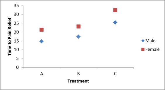
Notice that there is the same pattern of time to pain relief across treatments in both men and women (treatment effect). There is also a sex effect - specifically, time to pain relief is longer in women in every treatment.
Suppose that the same clinical trial is replicated in a second clinical site and the following data are observed.
Table - Time to Pain Relief by Treatment and Sex - Clinical Site 2
|
Treatment |
Male |
Female |
|---|---|---|
|
A |
22 |
21 |
|
25 |
19 |
|
|
26 |
18 |
|
|
27 |
24 |
|
|
24 |
25 |
|
|
B |
14 |
21 |
|
17 |
20 |
|
|
19 |
23 |
|
|
20 |
27 |
|
|
17 |
25 |
|
|
C |
15 |
37 |
|
17 |
34 |
|
|
19 |
36 |
|
|
14 |
26 |
|
|
12 |
29 |
The ANOVA table for the data measured in clinical site 2 is shown below.
Table - Summary of Two-Factor ANOVA - Clinical Site 2
|
Source of Variation |
Sums of Squares (SS) |
Degrees of freedom (df) |
Mean Squares (MS) |
F |
P-Value |
|---|---|---|---|---|---|
|
Model |
907.0 |
5 |
181.4 |
19.4 |
0.0001 |
|
Treatment |
71.5 |
2 |
35.7 |
3.8 |
0.0362 |
|
Sex |
313.6 |
1 |
313.6 |
33.5 |
0.0001 |
|
Treatment * Sex |
521.9 |
2 |
260.9 |
27.9 |
0.0001 |
|
Error or Residual |
224.4 |
24 |
9.4 |
||
|
Total |
1131.4 |
29 |
Notice that the overall test is significant (F=19.4, p=0.0001), there is a significant treatment effect, sex effect and a highly significant interaction effect. The table below contains the mean times to relief in each of the treatments for men and women.
Table - Mean Time to Pain Relief by Treatment and Gender - Clinical Site 2
|
Treatment |
Male |
Female |
|---|---|---|
|
A |
24.8 |
21.4 |
|
B |
17.4 |
23.2 |
|
C |
15.4 |
32.4 |
Notice that now the differences in mean time to pain relief among the treatments depend on sex. Among men, the mean time to pain relief is highest in Treatment A and lowest in Treatment C. Among women, the reverse is true. This is an interaction effect (see below).
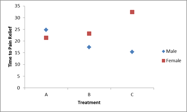
Notice above that the treatment effect varies depending on sex. Thus, we cannot summarize an overall treatment effect (in men, treatment C is best, in women, treatment A is best).
When interaction effects are present, some investigators do not examine main effects (i.e., do not test for treatment effect because the effect of treatment depends on sex). This issue is complex and is discussed in more detail in a later module.