


Sample Statistics
In order to illustrate the computation of sample statistics, we selected a small subset (n=10) of participants in the Framingham Heart Study. The data values for these ten individuals are shown in the table below. The rightmost column contains the body mass index (BMI) computed using the height and weight measurements. We will come back to this example in the module on Summarizing Data, but it provides a useful illustration of some of the terms that have been introduced and will also serve to illustrate the computation of some sample statistics.
Data Values for a Small Sample
|
Participant ID |
Systolic Blood Pressure |
Diastolic Blood Pressure |
Total Serum Cholesterol |
Weight |
Height |
Body Mass Index |
|---|---|---|---|---|---|---|
|
1 |
141 |
76 |
199 |
138 |
63.00 |
24.4 |
|
2 |
119 |
64 |
150 |
183 |
69.75 |
26.4 |
|
3 |
122 |
62 |
227 |
153 |
65.75 |
24.9 |
|
4 |
127 |
81 |
227 |
178 |
70.00 |
25.5 |
|
5 |
125 |
70 |
163 |
161 |
70.50 |
22.8 |
|
6 |
123 |
72 |
210 |
206 |
70.00 |
29.6 |
|
7 |
105 |
81 |
205 |
235 |
72.00 |
31.9 |
|
8 |
113 |
63 |
275 |
151 |
60.75 |
28.8 |
|
9 |
106 |
67 |
208 |
213 |
69.00 |
31.5 |
|
10 |
131 |
77 |
159 |
142 |
61.00 |
26.8 |
The first summary statistic that is important to report is the sample size. In this example the sample size is n=10. Because this sample is small (n=10), it is easy to summarize the sample by inspecting the observed values, for example, by listing the diastolic blood pressures in ascending order:
62 63 64 67 70 72 76 77 81 81
Simple inspection of this small sample gives us a sense of the center of the observed diastolic pressures and also gives us a sense of how much variability there is. However, for a large sample, inspection of the individual data values does not provide a meaningful summary, and summary statistics are necessary. The two key components of a useful summary for a continuous variable are:
- a description of the center or 'average' of the data (i.e., what is a typical value?) and
- an indication of the variability in the data.
Sample Mean
There are several statistics that describe the center of the data, but for now we will focus on the sample mean, which is computed by summing all of the values for a particular variable in the sample and dividing by the sample size. For the sample of diastolic blood pressures in the table above, the sample mean is computed as follows:

To simplify the formulas for sample statistics (and for population parameters), we usually denote the variable of interest as "X". X is simply a placeholder for the variable being analyzed. Here X=diastolic blood pressure.
The general formula for the sample mean is:

The X with the bar over it represents the sample mean, and it is read as "X bar". The Σ indicates summation (i.e., sum of the X's or sum of the diastolic blood pressures in this example).
When reporting summary statistics for a continuous variable, the convention is to report one more decimal place than the number of decimal places measured. Systolic and diastolic blood pressures, total serum cholesterol and weight were measured to the nearest integer, therefore the summary statistics are reported to the nearest tenth place. Height was measured to the nearest quarter inch (hundredths place), therefore the summary statistics are reported to the nearest thousandths place. Body mass index was computed to the nearest tenths place, summary statistics are reported to the nearest hundredths place.
Sample Variance and Standard Deviation
If there are no extreme or outlying values of the variable, the mean is the most appropriate summary of a typical value, and to summarize variability in the data we specifically estimate the variability in the sample around the sample mean. If all of the observed values in a sample are close to the sample mean, the standard deviation will be small (i.e., close to zero), and if the observed values vary widely around the sample mean, the standard deviation will be large. If all of the values in the sample are identical, the sample standard deviation will be zero.
When discussing the sample mean, we found that the sample mean for diastolic blood pressure = 71.3. The table below shows each of the observed values along with its respective deviation from the sample mean.

Table - Diastolic Blood Pressures and Deviations from the Sample Mean
|
X=Diastolic Blood Pressure |
Deviation from the Mean |
|---|---|
|
76 |
4.7 |
|
64 |
-7.3 |
|
62 |
-9.3 |
|
81 |
9.7 |
|
70 |
-1.3 |
|
72 |
0.7 |
|
81 |
9.7 |
|
63 |
-8.3 |
|
67 |
-4.3 |
|
77 |
5.7 |
|
|
|

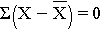
The deviations from the mean reflect how far each individual's diastolic blood pressure is from the mean diastolic blood pressure. The first participant's diastolic blood pressure is 4.7 units above the mean while the second participant's diastolic blood pressure is 7.3 units below the mean. What we need is a summary of these deviations from the mean, in particular a measure of how far, on average, each participant is from the mean diastolic blood pressure. If we compute the mean of the deviations by summing the deviations and dividing by the sample size we run into a problem. The sum of the deviations from the mean is zero. This will always be the case as it is a property of the sample mean, i.e., the sum of the deviations below the mean will always equal the sum of the deviations above the mean. However, the goal is to capture the magnitude of these deviations in a summary measure. To address this problem of the deviations summing to zero, we could take absolute values or square each deviation from the mean. Both methods would address the problem. The more popular method to summarize the deviations from the mean involves squaring the deviations (absolute values are difficult in mathematical proofs). The table below displays each of the observed values, the respective deviations from the sample mean and the squared deviations from the mean.
|
X=Diastolic Blood Pressure |
Deviation from the Mean
|
Squared Deviation from the Mean
|
|
76 |
4.7 |
22.09 |
|
64 |
-7.3 |
53.29 |
|
62 |
-9.3 |
86.49 |
|
81 |
9.7 |
94.09 |
|
70 |
-1.3 |
1.69 |
|
72 |
0.7 |
0.49 |
|
81 |
9.7 |
94.09 |
|
63 |
-8.3 |
68.89 |
|
67 |
-4.3 |
18.49 |
|
77 |
5.7 |
32.49 |
|
|
|
|


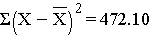
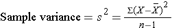
The squared deviations are interpreted as follows. The first participant's squared deviation is 22.09 meaning that his/her diastolic blood pressure is 22.09 units squared from the mean diastolic blood pressure, and the second participant's diastolic blood pressure is 53.29 units squared from the mean diastolic blood pressure. A quantity that is often used to measure variability in a sample is called the sample variance, and it is essentially the mean of the squared deviations. The sample variance is denoted s2 and is computed as follows:
|
Why do we divided by (n-1) instead of n? The sample variance is not actually the mean of the squared deviations, because we divide by (n-1) instead of n. In statistical inference (described in detail in another module) we make generalizations or estimates of population parameters based on sample statistics. If we were to compute the sample variance by taking the mean of the squared deviations and dividing by n we would consistently underestimate the true population variance. Dividing by (n-1) produces a better estimate of the population variance. The sample variance is nonetheless usually interpreted as the average squared deviation from the mean. |
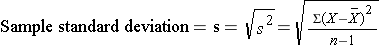
In this sample of n=10 diastolic blood pressures, the sample variance is s2 = 472.10/9 = 52.46. Thus, on average diastolic blood pressures are 52.46 units squared from the mean diastolic blood pressure. Because of the squaring, the variance is not particularly interpretable. The more common measure of variability in a sample is the sample standard deviation, defined as the square root of the sample variance:

A sample of 10 women seeking prenatal care at Boston Medical center agree to participate in a study to assess the quality of prenatal care. At the time of study enrollment, you the study coordinator, collected background characteristics on each of the moms including their age (in years).The data are shown below:
24 18 28 32 26 21 22 43 27 29


A sample of 12 men have been recruited into a study on the risk factors for cardiovascular disease. The following data are HDL cholesterol levels (mg/dL) at study enrollment:
50 45 67 82 44 51 64 105 56 60 74 68