


Effect Measure Modification
The term effect modification is applied to situations in which the magnitude of the effect of an exposure of interest differs depending on the level of a third variable. Reye's syndrome is a rare, but severe condition characterized by the sudden development of brain damage and liver dysfunction after a viral illness. The syndrome is most commonly seen in children between the ages of 4-14 who have been treated with aspirin while recovering from a viral illness, most commonly chickenpox or influenza. Fortunately, Reye's syndrome has become very uncommon since aspirin is no longer recommended for routine use in children. While Reye's syndrome can occur in adults, it is distinctly more common in children. Thus, the effect of aspirin treatment for a viral illness is very clearly modified by age.
In this situation, computing an overall estimate of association is misleading. One common way of dealing with effect modification is examine the association separately for each level of the third variable. For example, if one were to calculate the odds ratio for the association between aspirin treatment during a viral infection and development of Reye's syndrome, the odds ratio would be substantially greater in children than in adults. As another example, suppose a clinical trial is conducted and the drug is shown to result in a statistically significant reduction in total cholesterol. However, suppose that with closer scrutiny of the data, the investigators find that the drug is only effective in subjects with a specific genetic marker and that there is no effect in persons who do not possess the marker. The effect of the treatment is different depending on the presence or absence of the genetic marker. This is an example of effect modification or "statistical interaction".
Effect Modification with a Continuous Outcome
Evaluation of a Drug to Increase HDL Cholesterol
Consider the following clinical trial conducted to evaluate the efficacy of a new drug to increase HDL cholesterol (the "good" cholesterol). One hundred patients are enrolled in the trial and randomized to receive either the new drug or a placebo. Background characteristics (e.g., age, sex, educational level, income) and clinical characteristics (e.g., height, weight, blood pressure, total and HDL cholesterol levels) are measured at baseline, and they are found to be comparable in the two comparison groups. Subjects are instructed to take the assigned medication for 8 weeks, at which time their HDL cholesterol is measured again. The results are shown in the table below.
|
Sample Size |
Mean HDL |
Standard Deviation of HDL |
|
|---|---|---|---|
|
New Drug |
50 |
40.16 |
4.46 |
|
Placebo |
50 |
39.21 |
3.91 |
On average, the mean HDL levels are 0.95 units higher in patients treated with the new medication. A two sample test to compare mean HDL levels between treatments has a test statistic of Z = -1.13 which is not statistically significant at α=0.05.
Based on their preliminary studies, the investigators had expected a statistically significant increase in HDL cholesterol in the group treated with the new drug, and they wondered whether another variable might be masking the effect of the treatment. Other studies had, if fact, suggested that the effectiveness of a similar drug was différèrent in men and women. In this study, there are 19 men and 81 women. The table below shows the number and percent of men assigned to each treatment.
|
Sample Size |
Number (%) of Men |
|
|---|---|---|
|
New Drug |
50 |
0 (20%) |
|
Placebo |
50 |
9 (18%) |
There is no meaningful difference in the proportions of men assigned to receive the new drug or the placebo, so sex cannot be a confounder here, since it does not differed in the treatment groups. However, when the data are stratified by sex, they find the following:
| WOMEN |
Sample Size |
Mean HDL |
Standard Deviation of HDL |
|
New Drug |
40 |
38.88 |
3.97 |
|
Placebo |
41 |
39.24 |
4.21 |
|
|
|
|
|
|
MEN |
Sample Size |
Mean HDL |
Standard Deviation of HDL |
|
New Drug |
10 |
45.25 |
1.89 |
|
Placebo |
9 |
39.06 |
2.22 |
On average, the mean HDL levels are very similar in treated and untreated women, but the mean HDL levels are 6.19 units higher in men treated with the new drug. This is an example of effect modification by sex, i.e., the effect of the drug on HDL cholesterol is different for men and women. In this case there is no apparent effect in women, but there appears to be a moderately large effect in men. (Note, however, that the comparison in men is based on a very small sample size, so this difference should be interpreted cautiously, since it could be the result of random error or confounding.
When there is effect modification, analysis of the pooled data can be misleading. In this example, the pooled data (men and women combined), shows no effect of treatment. Because there is effect modification by sex, it is important to look at the differences in HDL levels among men and women, considered separately. In stratified analyses, however, investigators must be careful to ensure that the sample size is adequate to provide a meaningful analysis.
Effect Modification with a Dichotomous Outcome
Consider the following hypothetical study comparing hospitalization after a motor vehicle collision for male and female drivers.
Crude Data:
|
|
Hospitalized |
Not Hospitalized |
Total |
|---|---|---|---|
|
Male |
1330 |
7018 |
8348 |
|
Female |
798 |
6400 |
7198 |
Crude risk ratio=1.44
Age-Stratified:
Age ‹40
|
|
Hospitalized |
Not Hospitalized |
Total |
|---|---|---|---|
|
Male |
966 |
3146 |
4112 |
|
Female |
460 |
3000 |
3450 |
Stratum-specific risk ratio=1.80
Age ≥40
|
|
Hospitalized |
Not Hospitalized |
Total |
|---|---|---|---|
|
Male |
364 |
3872 |
4236 |
|
Female |
348 |
3400 |
3748 |
Stratum-specific risk ratio=0.93
In this case, the crude analysis suggests an association between male gender and frequency of hospitalization for motor vehicle collisions. However, if we stratify this by age, we see a strong association with male gender in subjects <40 years old, but no association in subjects 50+. Perhaps males <40 years old driver more recklessly than their female counterparts, but after age 40 driving aggression becomes similar in males and females.
Another good example of effect modification is seen with skin cancers. It is well established that excessive exposure to UV irradiation increases one's risk of skin cancer. However, the risk of UV-induced skin cancer is 1,000 times greater in people with xeroderma pigmentosum. This is a rate hereditary defect (autosomal recessive) in the enzyme system that repairs UV-induced damage to DNA. It is characterized by photosensitivity, pigmentary changes, premature skin aging, and greatly increased susceptibility to malignant tumor development.
If effect modification is present, it is NOT appropriate to use Mantel-Haenszel methods to combine the stratum-specific measures of association into a single pooled measurement. Effect modification is a biological phenomenon that should be described, so the stratum-specific estimates should be reported separately. In contrast, confounding is a distortion of the true association caused by an imbalance of some other risk factor.
- If there is only confounding: The stratum-specific measures of association will be similar to one another, but they will be different from the overall crude estimate by 10% or more. In this situation, one can use Mantel-Haenszel methods to calculate a pooled estimate (RR or OR) and p-value.
- If there is neither confounding nor effect modification: The crude estimate of association and the stratum-specific estimates will be similar. They don't have to be identical, just similar.
- If there is only effect modification: The stratum-specific estimates will differ from one another significantly. Whether they are "significantly different" can be tested by using a chi-square test of homogeneity
 , as described in the Aschengrau & Seage textbook.
 - If there is both effect modification and confounding: Here, you need to consider two possibilities:
1) If the stratum-specific estimates differ from one another, and they are both less than the crude estimate or if they are both greater than the crude estimate, then there is both confounding and effect modification.
2) If the stratum-specific estimates differ from one another, and the crude estimate is between the two stratum-specific estimates, then you need to pool the stratum-specific estimates (with a Mantel-Haenszel equation) to determine whether the pooled estimate is more than 10% different from the crude estimate.
Note that in this situation you are only pooling the stratum-specific estimates in order to make a decision about whether confounding is present; you should not report the pooled estimate as an "adjusted" measure of association if there is effect modification
Statistical Interaction versus Biological Interaction
While the discussion above provides a standard description of effect modification, but on closer scrutiny the concept of effect modification is more complicated than this. Consider the figure below (adapted from KJ Rothman: Epidemiology - An Introduction, Oxford University Press, 2002.) We see two scenarios in which incidence rates in exposed and unexposed individuals are assessed at different ages. Rate ratio and rate difference are both measures of effect, but depending on which we use, our conclusions about effect modification differ.
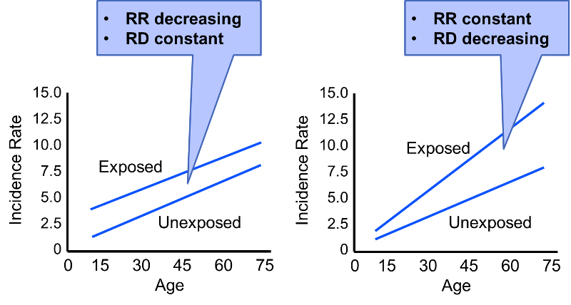
In the first scenario the rate difference remains constant across the spectrum of age, suggesting no effective modification. However, the rate ratio decreases with increasing age (RR=3 at age 15; RR=1.5 at age 75). In the second scenario the rate ratio remains relatively constant, but the rate difference increases with age. Our conclusion regarding whether or not there is effect modification will depend on which measure of effect we use.
Consider also the hypothetical data on the risk of lung cancer in smokers and non-smokers, both with and without exposure to asbestos (also adapted from Rothman).
Table - Hypothetical 1-Year Risk of Lung Cancer per 100,000
|
|
Without Asbestos |
With Asbestos Exposure |
|---|---|---|
|
Smokers |
5 |
50 |
|
Non-smokers |
1 |
10 |
First consider the effect of asbestos on the risk associated with smoking. The risk ratio is 5 both with and without asbestos exposure, suggesting no effect modification. However, the risk difference 4 per 100,000 without asbestosis and 40 per 100,000 with asbestosis exposure. This effect measure is clearly modified by asbestos. We can also look at the effect of smoking on the risk associated with asbestos. The risk ratio for asbestos exposure compared to no asbestos exposure is 10 in both smokers and non-smokers, suggesting an absence of effect modification. However, the risk difference is 45 per 100,000 in the presence of smoking, but only 9 per 100,000 in the absence of smoking. Thus, the risk ratios suggest no effect modification, but the risk differences suggest substantial effect modification.
Rothman argues that this ambiguity regarding effect measure modification and statistical interaction makes it important to make a distinction between statistical interaction (which is ambigous) and biological interaction (which is not ambiguous; it is either present or absent.) Biological interaction between two causes occurs if the effect of one is dependent on the presence of the other. For example, exposure to the measles virus is a component cause of developing measles, but it is dependent on another factor, i.e., the immune status of the exposed individual. Someone who is immune because of vaccination or having already had measles will not experience any effect from exposure to the measles virus. A discussion of the methods for measuring biological interaction is beyond the scope of this module. Those who are interested should refer to the discussion in Rothman's excellent text.

The director of the surgical trauma service at Boston Medical Center suspected that elderly drivers (age 70+) had inordinately poor outcomes compared to younger drivers after being in a motor vehicle collision (MVC). His research hypothesis was tested using data from the Boston Medical Center Trauma registry and data from the National Trauma Data Bank.
- Are there any factors that might confound the association between being al elderly driver and the risk of death after a motor vehicle collision? If so, what factors would you consider? How would you deal with these potential confounders?
- The figure below summarizes some of the data obtained from the Boston Medical Center Trauma registry. The upper contingency table shows deaths among the 74 elderly drivers hospitalized after an MVC and the 960 younger drivers who had been hospitalized after an MVC. The lower two tables summarize the findings after stratifying based on whether the drivers had the benefit of safety devices (seat belt buckled and/or air bag in the vehicle. Do these findings suggest the presence of effect modification? Why or why not?
Crude Analysis:
|
|
Died |
Lived |
Total |
|---|---|---|---|
|
Age ≥70 |
13 |
61 |
74 |
|
Age‹70 |
25 |
935 |
960 |
Stratified by Use of a Safety Restraint:
Unrestrained (no seatbelt or air bag):
|
|
Died |
Lived |
Total |
|---|---|---|---|
|
Age ≥70 |
8 |
16 |
24 |
|
Age‹70 |
13 |
359 |
372 |
Restrained with Seatbelt, Air Bag, or Both
|
|
Died |
Lived |
Total |
|---|---|---|---|
|
Age ≥70 |
5 |
45 |
50 |
|
Age‹70 |
12 |
576 |
588 |
Try to answer these questions on your own. Then proceed to the next page to see the answers.